Thermal Analysis

Thermal analysis of a simple construction.

• use SolidBodyThermal and SolidBodySurfaceHeatTransfer

• evaluate the surface heat flux at internal and external boundaries with a job Plugin

• view the temperature field

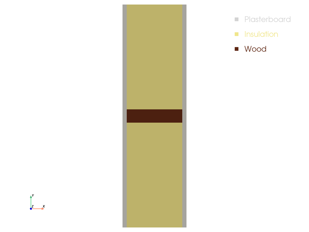
This example describes a simple two-dimensional light-weight construction system set up with three solids. The temperature boundary conditions have a \(\pm 1\) K sinusoidal variation around their average value with a period of 24 h.

import matplotlib.pyplot as plt
import numpy as np

import felupe as fem

Define material properties as lists for plasterboard, insulation and wood. This includes mass density, specific heat capacity and thermal conductivity.

density = [1000, 20, 500]  # kg/m^3
specific_heat = [1125, 1450, 1600]  # J/(kg K)
thermal_conductivity = [0.4, 0.035, 0.16]  # W/(m K)

Set up one mesh per material. If a material consists of multiple areas, the separate rectangles are collected in a mesh container and are merged into one mesh per material. These meshes per material are then added to a mesh container for the construction.

plasterboard_1 = fem.Rectangle(b=(0.018, 0.47), n=(6, 18))  # bottom left
plasterboard_2 = fem.Rectangle(a=(0.0, 0.47), b=(0.018, 0.53), n=(11, 7))  # center left
plasterboards = fem.MeshContainer(
    [
        plasterboard_1,  # bottom left
        plasterboard_1.translate(0.268, axis=0),  # bottom right
        plasterboard_1.translate(0.53, axis=1),  # top left
        plasterboard_1.translate(0.268, axis=0).translate(0.53, axis=1),  # top right
        plasterboard_2,  # center left
        plasterboard_2.translate(0.268, axis=0),  # center right
    ],
    merge=True,
).stack()

insulation = fem.Rectangle(a=(0.018, 0), b=(0.268, 0.47), n=(12, 18))  # bottom
insulations = fem.MeshContainer(
    [
        insulation,
        insulation.translate(0.53, axis=1),
    ],
    merge=True,
).stack()

wood = fem.Rectangle(a=(0.018, 0.47), b=(0.268, 0.53), n=(12, 8))
container = fem.MeshContainer([plasterboards, insulations, wood], merge=True)

container.plot(
    colors=["lightgrey", "khaki", "sepia"],
    labels=["Plasterboard", "Insulation", "Wood"],
    show_edges=False,
).show()

Static Scene

Interactive Scene

A top-level temperature field is defined on the whole construction with an initial temperature value of 10 °C, and separate fields are defined for each material. The surface heat transfer coefficients and ambient temperatures are defined for the internal and external boundaries. Thermal solid bodies are created for each material.

regions = [fem.RegionQuad(m) for m in container]
fields = [fem.Field(r, dim=1).as_container() for r in regions]

# top level temperature field
mesh = container.stack()
region = fem.RegionQuad(mesh)
temperature = fem.Field(region, dim=1, values=10.0)  # initial temperature 10 °C
field = fem.FieldContainer([temperature])

external_region = fem.RegionQuadBoundary(mesh, mask=mesh.x == mesh.x.min())
external_temperature = fem.Field(external_region, dim=1)
external_field = fem.FieldContainer([external_temperature])

internal_region = fem.RegionQuadBoundary(mesh, mask=mesh.x == mesh.x.max())
internal_temperature = fem.Field(internal_region, dim=1)
internal_field = fem.FieldContainer([internal_temperature])

external_heat_transfer = fem.thermal.SolidBodySurfaceHeatTransfer(
    field=external_field,
    coefficient=25.0,  # W/(m^2 K)
    temperature=0.0,  # °C
)
internal_heat_transfer = fem.thermal.SolidBodySurfaceHeatTransfer(
    field=internal_field,
    coefficient=7.69,  # W/(m^2 K)
    temperature=20.0,  # °C
)

materials = []
for mfield, rho, cp, k in zip(fields, density, specific_heat, thermal_conductivity):
    materials.append(
        fem.thermal.SolidBodyThermal(
            field=mfield,
            mass_density=rho,
            specific_heat_capacity=cp,
            thermal_conductivity=k,
        )
    )

A callback-function records the mean surface heat flux at the internal and external boundaries after each completed time step. The mean surface heat flux is calculated by the heat_flux_boundary() method of the thermal solid body, which returns the integrated surface heat flux for a given boundary region and time step. The mean surface heat flux is stored in the flux_data dictionary, which is passed to the callback function as an argument.

def callback(stepnumber, substepnumber, substep, flux_data):
    """Save mean surface heat flux at internal and external boundaries."""

    heat_flux = materials[0].heat_flux_boundary
    flux_data["external"].append(heat_flux(region=external_region))
    flux_data["internal"].append(heat_flux(region=internal_region))


time_steps = fem.math.linsteps([0, 24 * 3600], num=int(24 * 3600 / 720))[1:]

t_ext = 0 + 1 * np.sin(2 * np.pi * time_steps / 86400)
t_int = 20 + 1 * np.sin(2 * np.pi * time_steps / 86400)

The time step item is created with the thermal solid bodies. It must be located as the first item in the step to properly update the time step in the materials. The internal and external heat transfer item values are defined in the ramp, which specifies how their values change over time. Finally, a job is created with the step and the callback function, and evaluated with the top-level temperature field. A result file is created for visualization in Paraview, and the temperature field is saved as point- data in the result file.

time = fem.thermal.TimeStep(
    [*materials, external_heat_transfer, internal_heat_transfer]
)
ramp = {
    time: time_steps,
    internal_heat_transfer: t_int,
    external_heat_transfer: t_ext,
}
step = fem.Step(
    items=[time, *materials, internal_heat_transfer, external_heat_transfer],
    ramp=ramp,
)

flux_data = {"external": [], "internal": []}

job = fem.Job(steps=[step], callback=callback, flux_data=flux_data).evaluate(
    x0=field,
    filename="result.xdmf",  # create a result file for Paraview
    point_data={"Temperature": lambda field, substep: temperature.values},
    point_data_default=False,
    cell_data_default=False,
)

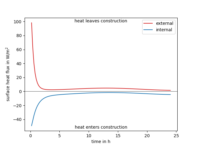
Internal and external surface heat flux values are plotted over time.

注釈

The heat flux is positive when heat leaves the construction (here, on the external surface), and negative when heat enters the construction (here, on the internal surface).

fig, ax = plt.subplots()
ax.plot(time_steps / 3600, flux_data["external"], color="C3", label="external")
ax.plot(time_steps / 3600, flux_data["internal"], color="C0", label="internal")

tmin, tmax = ax.get_xlim()
ax.plot([tmin, tmax], np.zeros(2), "black", lw=0.5)

text_kwargs = dict(transform=ax.transAxes, ha="center", va="center")
ax.text(0.5, 0.97, "heat leaves construction", **text_kwargs)
ax.text(0.5, 0.03, "heat enters construction", **text_kwargs)

ax.legend()
ax.set(xlim=(tmin, tmax), xlabel="time in h", ylabel=r"surface heat flux in W/m$^2$")

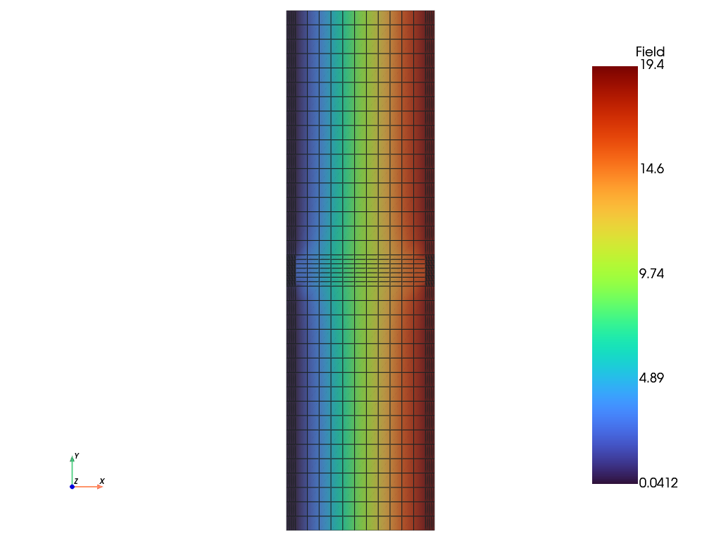
A view on the temperature field at the end of the simulation period visualizes the temperature distribution.

field.plot("Field", scalar_bar_vertical=True).show()

Static Scene

Interactive Scene