Mechanics

Solid Bodies

SolidBody(umat, field[, statevars, density, ...])	A SolidBody with methods for the assembly of sparse vectors/matrices.
SolidBodyNearlyIncompressible(umat, field, bulk)	A (nearly) incompressible solid body with methods for the assembly of sparse vectors/matrices.
SolidBodyForce(field[, values, scale])	A body force on a solid body.
SolidBodyPressure(field[, pressure])	A hydrostatic pressure boundary on a solid body.
SolidBodyCauchyStress(field[, cauchy_stress])	A Cauchy stress boundary on a solid body.
TrussBody(umat, field, area[, statevars])	A Truss body with methods for the assembly of sparse vectors/matrices.

Steps and Jobs

Step(items[, ramp, boundaries])	A Step with multiple substeps, subsequently depending on the solution of the previous substep.
Job(steps[, callback, plugins])	A job with a list of steps and a method to evaluate them.
CharacteristicCurve(steps, boundary[, ...])	A job with a list of steps and a method to evaluate them.
FreeVibration(items[, boundaries])	A Free-Vibration Step/Job.

Job Plugins

Plugin()	Base class for plugins.
AnimationWriterPlugin(items[, filename, ...])	A job plugin to write an animation file during job evaluation.
CharacteristicCurvePlugin(boundary[, items])	A job plugin to record a characteristic curve.
ProgressPlugin([verbose, tqdm])	A job plugin to output the progress of a job evaluation in the terminal.
XDMFWriterPlugin([filename, mesh, ...])	A job plugin to write XDMF files during job evaluation.
EventDispatcher([plugins])	A class to dispatch events to plugins during evaluation.
Context([job, step, substep])	A class to keep track of the context of a Job during evaluation.
JobState([stepnumber, substepnumber, time])	A class to keep track of the state of a Job during evaluation.
IterationState([iteration, fnorm, xnorm, ...])	A class to keep track of the state of an iteration during evaluation.

Point Load and Multi-Point Constraints

PointLoad(field, points[, values, apply_on, ...])	A point load with methods for the assembly of sparse vectors/matrices, applied on the n-th field.
MultiPointConstraint(field, points, centerpoint)	A Multi-point-constraint which connects a center-point to a list of points.
MultiPointContact(field, points, centerpoint)	A frictionless point-to-rigid (wall) contact which connects a center-point to a list of points.

Contact

ContactRigidPlane(field, points, ...[, ...])

A node-to-surface contact, where the surface is given by a rigid plane.

Helpers for Custom Items and State Variables

mechanics.StateNearlyIncompressible(field)	A State with internal cell-wise constant dual fields for (nearly) incompressible solid bodies.
mechanics.Assemble([vector, matrix, mass, ...])	A class with methods for assembling vectors and matrices of an Item.
mechanics.Evaluate(gradient, hessian[, ...])	A class with evaluate methods of an Item.
mechanics.Results([stress, elasticity])	A class with intermediate results of an Item.
mechanics.UpdateItem(parent, key)	A helper class to update an item in the parent class when the value changes.

Detailed API Reference

class felupe.SolidBody(umat, field, statevars=None, density=None, block=True, apply=None, multiplier=None)

ベースクラス: Solid

A SolidBody with methods for the assembly of sparse vectors/matrices.

パラメータ:

• umat (class) -- A class which provides methods for evaluating the gradient and the hessian of the strain energy density function per unit undeformed volume. The function signatures must be dψdF, ζ_new = umat.gradient([F, ζ]) for the gradient and d2ψdFdF = umat.hessian([F, ζ]) for the hessian of the strain energy density function \(\psi(\boldsymbol{F})\), where \(\boldsymbol{F}\) is the deformation gradient tensor and \(\zeta\) holds the array of internal state variables.

• field (FieldContainer) -- A field container with one or more fields.

• statevars (ndarray or None, optional) -- Array of initial internal state variables (default is None).

• density (float or None, optional) -- The density of the solid body.

• block (bool, optional) -- Assemble a sparse matrix from sparse sub-blocks or assemble a sparse vector by stacking sparse matrices vertically (row wise). Default is True.

• apply (callable or None, optional) -- Apply a callable on the assembled vectors and sparse matrices. Default is None.

• multiplier (float or None, optional) -- A scale factor for the assembled vector and matrix. Default is None.

メモ

The total potential energy of internal forces is given in Eq. (1)

(1)\[\Pi_{int}(\boldsymbol{F}) = \int_V \psi(\boldsymbol{F})\ dV\]

with its variation, see Eq. (2)

(2)\[\delta_\boldsymbol{u}(\Pi_{int}) = \int_V \frac{\partial \psi}{\partial \boldsymbol{F}} \ dV \longrightarrow \boldsymbol{f}_\boldsymbol{u}\]

and linearization, see Eq. (3). The right-arrows in Eq. (2) and Eq. (3) represent the assembly into system scalars, vectors or matrices.

(3)\[\delta_\boldsymbol{u}\Delta_\boldsymbol{u}(\Pi_{int}) = \int_V \delta\boldsymbol{F} : \frac{\partial^2 \psi}{ \partial \boldsymbol{F}\ \partial \boldsymbol{F} } : \Delta\boldsymbol{F}\ dV \longrightarrow \boldsymbol{K}_{\boldsymbol{u}\boldsymbol{u}}\]

The displacement-based formulation leads to a linearized equation system as given in Eq. (4).

(4)\[\boldsymbol{K}_{\boldsymbol{u}\boldsymbol{u}} \cdot \delta \boldsymbol{u} + \boldsymbol{f}_\boldsymbol{u} = \boldsymbol{0}\]

注釈

This class also supports umat with mixed-field formulations like NearlyIncompressible or ThreeFieldVariation.

サンプル

>>> import felupe as fem
>>>
>>> mesh = fem.Cube(n=6)
>>> region = fem.RegionHexahedron(mesh)
>>> field = fem.FieldContainer([fem.Field(region, dim=3)])
>>> boundaries = fem.dof.uniaxial(field, clamped=True, return_loadcase=False)
>>>
>>> umat = fem.NeoHooke(mu=1, bulk=2)
>>> solid = fem.SolidBody(umat, field)
>>>
>>> table = fem.math.linsteps([0, 1], num=5)
>>> step = fem.Step(
...     items=[solid],
...     ramp={boundaries["move"]: table},
...     boundaries=boundaries,
... )
>>>
>>> job = fem.Job(steps=[step]).evaluate()
>>> solid.plot("Principal Values of Cauchy Stress").show()

参考

felupe.SolidBodyNearlyIncompressible

A (nearly) incompressible solid body with methods for the assembly of sparse vectors/matrices.

checkpoint()

Return a checkpoint of the solid body.

戻り値:

A dict with checkpoint arrays / objects.

戻り値の型:

dict

サンプル

import felupe as fem

mesh = fem.Rectangle(b=(3, 1), n=(7, 3))
region = fem.RegionQuad(mesh)
field = fem.FieldContainer([fem.FieldPlaneStrain(region, dim=2)])

umat = fem.NeoHooke(mu=1, bulk=2)
solid = fem.SolidBody(umat=umat, field=field)

# 1. vertical compression
boundaries = fem.dof.uniaxial(
    field, clamped=True, sym=False, axis=1, return_loadcase=False
)
ramp = {boundaries["move"]: fem.math.linsteps([0, -0.2], num=2)}
step = fem.Step(items=[solid], ramp=ramp, boundaries=boundaries)
job = fem.Job(steps=[step]).evaluate()

# checkpoint the current state of deformation
checkpoint = solid.checkpoint()

# 2a. horizontal shear (right)
boundaries = fem.dof.shear(
    field, sym=False, moves=(0, 0, -0.2), return_loadcase=False
)
ramp = {boundaries["move"]: fem.math.linsteps([0, 1], num=2)}
step = fem.Step(items=[solid], ramp=ramp, boundaries=boundaries)
job = fem.Job(steps=[step]).evaluate()

# (1.) restore compression without shear
solid.restore(checkpoint)

# 2b. horizontal shear (left)
boundaries = fem.dof.shear(
    field, sym=False, moves=(0, 0, -0.2), return_loadcase=False
)
ramp = {boundaries["move"]: fem.math.linsteps([0, -1], num=2)}
step = fem.Step(items=[solid], ramp=ramp, boundaries=boundaries)
job = fem.Job(steps=[step]).evaluate()

参考

felupe.SolidBody.restore

Restore a checkpoint of a solid body inplace.

restore(checkpoint, restore_statevars=True)

Restore a checkpoint inplace.

パラメータ:

• checkpoint (dict) -- A dict with checkpoint arrays / objects.

• restore_statevars (bool, optional) -- Flag to restore state variables. This is a power feature and must be used with caution! Default is True.

参考

felupe.SolidBody.checkpoint

Return a checkpoint of the solid body.

revolve(n=11, phi=180)

Return a revolved solid body.

パラメータ:

• n (int, optional) -- Number of n-point revolutions (or (n-1) cell revolutions), default is 11.

• phi (float or ndarray, optional) -- Revolution angle in degree (default is 180).

戻り値:

The revolved solid body.

戻り値の型:

SolidBody

サンプル

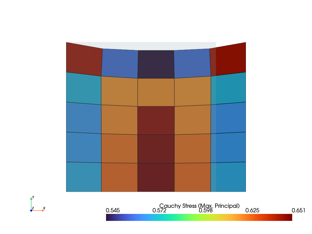
First, create an axisymmetric model. A non-homogeneous uniaxial tension load case is applied on the solid body.

>>> import felupe as fem
>>>
>>> region = fem.RegionQuad(mesh=fem.Rectangle(n=6))
>>> field = fem.FieldContainer([fem.FieldAxisymmetric(region, dim=2)])
>>>
>>> umat = fem.NeoHookeCompressible(mu=1, lmbda=2)
>>> solid = fem.SolidBody(umat=umat, field=field)
>>>
>>> boundaries = fem.dof.uniaxial(
...     solid.field, clamped=True, sym=False, return_loadcase=False
... )
>>> step = fem.Step(items=[solid], boundaries=boundaries)
>>> job = fem.Job(steps=[step]).evaluate()
>>>
>>> solid.plot("Principal Values of Cauchy Stress").show()

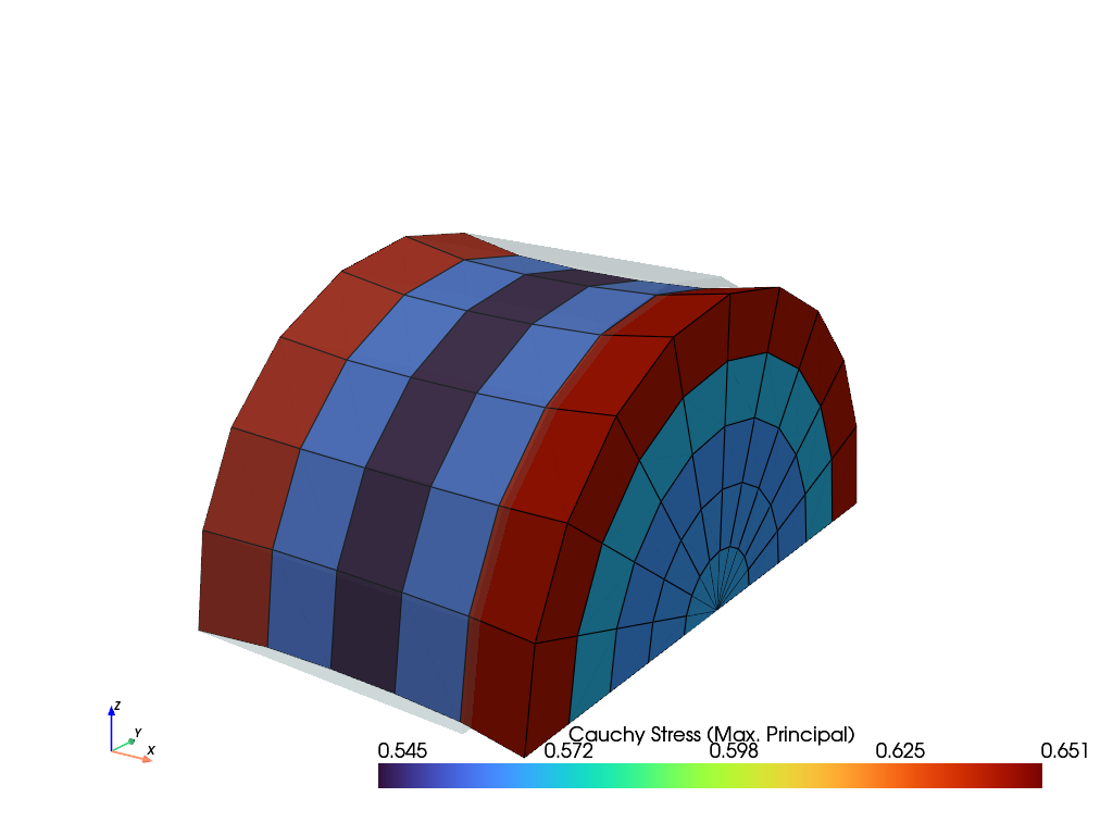
The solid body is now revolved around the x-axis. This model may now be used to apply non-axisymmetric loads. Here, the same load case is also applied on the 3d-model.

>>> new_solid = solid.revolve(n=11, phi=180)
>>> boundaries = fem.dof.uniaxial(
...     new_solid.field, clamped=True, sym=(0, 0, 1), return_loadcase=False
... )
>>>
>>> step = fem.Step(items=[new_solid], boundaries=boundaries)
>>> job = fem.Job(steps=[step]).evaluate()
>>>
>>> new_solid.plot("Principal Values of Cauchy Stress").show()

参考

SolidBodyNearlyIncompressible.revolve

Return a revolved solid body

class felupe.SolidBodyNearlyIncompressible(umat, field, bulk, state=None, statevars=None, density=None)

ベースクラス: Solid

A (nearly) incompressible solid body with methods for the assembly of sparse vectors/matrices. The constitutive material definition must provide the distortional part of the strain energy density function per unit undeformed volume only. The volumetric part of the strain energy density function is automatically added on additional internal (dual) cell-wise constant fields.

パラメータ:

• umat (class) -- A class which provides methods for evaluating the gradient and the hessian of the isochoric part of the strain energy density function per unit undeformed volume \(\hat\psi(\boldsymbol{F})\). The function signatures must be dψdF, ζ_new = umat.gradient([F, ζ]) for the gradient and d2ψdFdF = umat.hessian([F, ζ]) for the hessian of the strain energy density function \(\hat{\psi}(\boldsymbol{F})\), where \(\boldsymbol{F}\) is the deformation gradient tensor and \(\zeta\) holds the array of internal state variables.

• field (FieldContainer) -- A field container with one or more fields.

• bulk (float) -- The bulk modulus of the volumetric part of the strain energy function \(U(\bar{J})=K(\bar{J}-1)^2/2\).

• state (StateNearlyIncompressible or None, optional) -- A valid initial state for a (nearly) incompressible solid (default is None).

• statevars (ndarray or None, optional) -- Array of initial internal state variables (default is None).

• density (float or None, optional) -- The density of the solid body.

メモ

注釈

This nearly-incompressible solid body works best with RegionQuad and RegionHexahedron regions. RegionQuadraticTriangle and RegionQuadraticTetra regions are also supported.

The total potential energy of internal forces for a three-field variational approach, suitable for nearly-incompressible material behaviour, is given in Eq. (5)

(5)\[\Pi_{int}(\boldsymbol{F}, p, \bar{J}) = \int_V \hat{\psi}(\boldsymbol{F})\ dV + \int_V U(\bar{J})\ dV + \int_V p (J - \bar{J})\ dV\]

with its variations, see Eq. (6)

(6)\[ \begin{align}\begin{aligned}\delta_\boldsymbol{u}(\Pi_{int}) &= \int_V \left( \frac{\partial \hat{\psi}}{\partial \boldsymbol{F}} + p\ \frac{\partial J}{\partial \boldsymbol{F}} \right) : \delta\boldsymbol{F}\ dV \longrightarrow \boldsymbol{r}_\boldsymbol{u}\\\delta_p(\Pi_{int}) &= \int_V \left( J - \bar{J} \right)\ \delta p\ dV \longrightarrow r_p\\\delta_\bar{J}(\Pi_{int}) &= \int_V \left( K \left( \bar{J} - 1 \right) - p \right)\ \delta \bar{J}\ dV \longrightarrow r_{\bar{J}}\end{aligned}\end{align} \]

and linearizations, see Eq. (7) [1] [2] [3]. The right-arrows in Eq. (6) and Eq. (7) represent the assembly into system scalars, vectors or matrices.

(7)\[ \begin{align}\begin{aligned}\delta_\boldsymbol{u}\Delta_\boldsymbol{u}(\Pi_{int}) &= \int_V \delta\boldsymbol{F} : \left( \frac{\partial^2 \hat{\psi}}{ \partial \boldsymbol{F}\ \partial \boldsymbol{F} } + p \frac{\partial^2 J}{\partial \boldsymbol{F}\ \partial \boldsymbol{F}} \right) : \Delta\boldsymbol{F}\ dV \longrightarrow \boldsymbol{K}_{\boldsymbol{u}\boldsymbol{u}}\\\delta_\boldsymbol{u}\Delta_p(\Pi_{int}) &= \int_V \delta \boldsymbol{F} : \frac{\partial J}{\partial \boldsymbol{F}}\ \Delta p\ dV \longrightarrow \boldsymbol{K}_{\boldsymbol{u}p}\\\delta_p\Delta_{\bar{J}}(\Pi_{int}) &= \int_V \delta p\ (-1)\ \Delta \bar{J}\ dV \longrightarrow -V\\\delta_{\bar{J}}\Delta_{\bar{J}}(\Pi_{int}) &= \int_V \delta \bar{J}\ K\ \Delta \bar{J}\ dV \longrightarrow K\ V\end{aligned}\end{align} \]

The assembled constraint equations for the variations w.r.t. the dual fields \(p\) and \(\bar{J}\) are given in Eq. (8).

(8)\[ \begin{align}\begin{aligned}r_p &= \left( \frac{v}{V} - \bar{J} \right) V\\r_{\bar{J}} &= \left( K (\bar{J} - 1) - p \right) V\end{aligned}\end{align} \]

The volumetric part of the strain energy density function is denoted in Eq. (9) along with its first and second derivatives.

(9)\[ \begin{align}\begin{aligned}\bar{U} &= \frac{K}{2} \left( \bar{J} - 1 \right)^2\\\bar{U}' &= K \left( \bar{J} - 1 \right)\\\bar{U}'' &= K\end{aligned}\end{align} \]

Hu-Washizu Three-Field-Variational Principle

The Three-Field-Variation \((\boldsymbol{u},p,\bar{J})\) leads to a linearized equation system with nine sub block-matrices, see Eq. (10) [4]. Due to the fact that the equation system is derived by a potential, the matrix is symmetric and hence, only six independent sub-matrices have to be evaluated. Furthermore, by the application of the mean dilatation technique, two of the remaining six sub-matrices are identified to be zero. That means four sub-matrices are left to be evaluated, where two non-zero sub-matrices are scalar-valued entries.

(10)\[\begin{split}\begin{bmatrix} \boldsymbol{K}_{\boldsymbol{u}\boldsymbol{u}} & \boldsymbol{K}_{\boldsymbol{u}p} & \boldsymbol{0} \\ \boldsymbol{K}_{\boldsymbol{u}p}^T & 0 & -V \\ \boldsymbol{0}^T & -V & K\ V \end{bmatrix} \cdot \begin{bmatrix} \delta \boldsymbol{u} \\ \delta p \\ \delta \bar{J} \end{bmatrix} + \begin{bmatrix} \boldsymbol{r}_\boldsymbol{u} \\ r_p \\ r_\bar{J} \end{bmatrix} = \begin{bmatrix} \boldsymbol{0}\\ 0 \\ 0 \end{bmatrix}\end{split}\]

A condensed representation of the equation system, only dependent on the primary unknowns \(\boldsymbol{u}\) is carried out. To do so, the second line is multiplied by the bulk modulus \(K\), see Eq. (11).

(11)\[\begin{split}\begin{bmatrix} \boldsymbol{K}_{\boldsymbol{u}\boldsymbol{u}} & \boldsymbol{K}_{\boldsymbol{u}p} & \boldsymbol{0} \\ K \boldsymbol{K}_{\boldsymbol{u}p}^T & 0 & -K\ V \\ \boldsymbol{0}^T & -V & K\ V \end{bmatrix} \cdot \begin{bmatrix} \delta \boldsymbol{u} \\ \delta p \\ \delta \bar{J} \end{bmatrix} + \begin{bmatrix} \boldsymbol{r}_\boldsymbol{u} \\ K\ r_p \\ r_\bar{J} \end{bmatrix} = \begin{bmatrix} \boldsymbol{0}\\ 0 \\ 0 \end{bmatrix}\end{split}\]

Lines two and three are contracted by summation as given in Eq. (12). This eliminates \(\bar{J}\) from the unknowns.

(12)\[\begin{split}\begin{bmatrix} \boldsymbol{K}_{\boldsymbol{u}\boldsymbol{u}} & \boldsymbol{K}_{\boldsymbol{u}p} \\ K \boldsymbol{K}_{\boldsymbol{u}p}^T & -V \end{bmatrix} \cdot \begin{bmatrix} \delta \boldsymbol{u} \\ \delta p \end{bmatrix} + \begin{bmatrix} \boldsymbol{r}_\boldsymbol{u} \\ K\ r_p + r_\bar{J} \end{bmatrix} = \begin{bmatrix} \boldsymbol{0}\\ 0 \end{bmatrix}\end{split}\]

Next, the second line is left-expanded by \(\frac{1}{V}~\boldsymbol{K}_{\boldsymbol{u}p}\) and both equations are summed up again, see (13).

(13)\[\left( \boldsymbol{K}_{\boldsymbol{u}\boldsymbol{u}} + \frac{K}{V}~\boldsymbol{K}_{\boldsymbol{u}p} \otimes \boldsymbol{K}_{\boldsymbol{u}p} \right) \cdot \delta \boldsymbol{u} + \boldsymbol{r}_\boldsymbol{u} + \frac{K~r_p + r_\bar{J}}{V} \boldsymbol{K}_{\boldsymbol{u}p} = \boldsymbol{0}\]

The secondary unknowns are evaluated after solving the primary unknowns, see Eq. (14).

(14)\[ \begin{align}\begin{aligned}\delta \bar{J} &= \frac{1}{V} \delta \boldsymbol{u} \cdot \boldsymbol{K}_{\boldsymbol{u}p} + \frac{v}{V} - \bar{J}\\\delta p &= K \left(\bar{J} + \delta \bar{J} - 1 \right) - p\end{aligned}\end{align} \]

The condensed constraint equation in Eq. (13) is given in Eq. (15)

(15)\[\frac{K~r_p + r_{\bar{J}}}{V} = K \left( \frac{v}{V} - 1 \right) - p\]

and the deformed volume is evaluated by Eq. (16).

(16)\[v = \int_V J\ dV\]

サンプル

>>> import felupe as fem
>>>
>>> mesh = fem.Cube(n=6)
>>> region = fem.RegionHexahedron(mesh)
>>> field = fem.FieldContainer([fem.Field(region, dim=3)])
>>> boundaries = fem.dof.uniaxial(field, clamped=True, return_loadcase=False)
>>>
>>> umat = fem.NeoHooke(mu=1)
>>> solid = fem.SolidBodyNearlyIncompressible(umat, field, bulk=5000)
>>>
>>> table = fem.math.linsteps([0, 1], num=5)
>>> step = fem.Step(
...     items=[solid],
...     ramp={boundaries["move"]: table},
...     boundaries=boundaries,
... )
>>>
>>> job = fem.Job(steps=[step]).evaluate()
>>> solid.plot("Principal Values of Cauchy Stress").show()

参照

[1]

J. Bonet, A. J. Gil, and R. D. Wood, "Nonlinear Solid Mechanics for Finite Element Analysis: Statics". Cambridge University Press, Jun. 05, 2016. doi: 10.1017/cbo9781316336144.

[2]

O. C. Zienkiewicz, R. L. Taylor and J.Z. Zhu, "The Finite Element Method: its Basis and Fundamentals". Elsevier, 2013. doi: 10.1016/c2009-0-24909-9.

[3]

G. A. Holzapfel, "Nonlinear Solid Mechanics. A Continuum Approach for Engineering". Wiley, 2000. isbn: 047182304X.

[4]

J. A. Schönherr, P. Schneider, and C. Mittelstedt, "Robust hybrid/mixed finite elements for rubber-like materials under severe compression", Computational Mechanics, vol. 70, no. 1. Springer Science and Business Media LLC, pp. 101–122, Mar. 31, 2022. doi: 10.1007/s00466-022-02157-y.

参考

felupe.StateNearlyIncompressible

A State with internal cell-wise constant fields for (nearly) incompressible solid bodies.

checkpoint()

Return a checkpoint of the nearly-incompressible solid body.

戻り値:

A dict with checkpoint arrays / objects.

戻り値の型:

dict

サンプル

import felupe as fem

mesh = fem.Rectangle(b=(3, 1), n=(7, 3))
region = fem.RegionQuad(mesh)
field = fem.FieldContainer([fem.FieldPlaneStrain(region, dim=2)])

umat = fem.NeoHooke(mu=1)
solid = fem.SolidBodyNearlyIncompressible(umat=umat, field=field, bulk=5000)

# 1. vertical compression
boundaries = fem.dof.uniaxial(
    field, clamped=True, sym=False, axis=1, return_loadcase=False
)
ramp = {boundaries["move"]: fem.math.linsteps([0, -0.2], num=2)}
step = fem.Step(items=[solid], ramp=ramp, boundaries=boundaries)
job = fem.Job(steps=[step]).evaluate()

# checkpoint the current state of deformation
checkpoint = solid.checkpoint()

# 2a. horizontal shear (right)
boundaries = fem.dof.shear(
    field, sym=False, moves=(0, 0, -0.2), return_loadcase=False
)
ramp = {boundaries["move"]: fem.math.linsteps([0, 1], num=2)}
step = fem.Step(items=[solid], ramp=ramp, boundaries=boundaries)
job = fem.Job(steps=[step]).evaluate()

# (1.) restore compression without shear
solid.restore(checkpoint)

# 2b. horizontal shear (left)
boundaries = fem.dof.shear(
    field, sym=False, moves=(0, 0, -0.2), return_loadcase=False
)
ramp = {boundaries["move"]: fem.math.linsteps([0, -1], num=2)}
step = fem.Step(items=[solid], ramp=ramp, boundaries=boundaries)
job = fem.Job(steps=[step]).evaluate()

参考

felupe.SolidBody.restore

Restore a checkpoint of a nearly-incompressible solid body inplace.

restore(checkpoint, restore_statevars=True, restore_state=True)

Restore a checkpoint inplace.

パラメータ:

• checkpoint (dict) -- A dict with checkpoint arrays / objects.

• restore_statevars (bool, optional) -- Flag to restore state variables. This is a power feature and must be used with caution! Default is True.

参考

felupe.SolidBodyNearlyIncompressible.checkpoint

Return a checkpoint of the nearly-incompressible solid body.

revolve(n=11, phi=180)

Return a revolved solid body.

パラメータ:

• n (int, optional) -- Number of n-point revolutions (or (n-1) cell revolutions), default is 11.

• phi (float or ndarray, optional) -- Revolution angle in degree (default is 180).

戻り値:

The revolved solid body.

戻り値の型:

SolidBody

参考

SolidBody.revolve

Return a revolved solid body

class felupe.SolidBodyForce(field, values=None, scale=1.0)

ベースクラス: object

A body force on a solid body.

パラメータ:

• field (FieldContainer) -- A field container with fields created on a boundary region.

• values (ndarray or None, optional) -- The prescribed values (e.g. gravity \(\boldsymbol{g}\)). Default is None. If None, the values are set to zero (the dimension is derived from the first field of the field container).

• scale (float, optional) -- An optional scale factor for the values, e.g. density \(\rho\) of the solid body. Default is 1.0.

メモ

\[\delta W_{ext} = \int_V \delta \boldsymbol{u} \cdot \rho \boldsymbol{g} \ dV\]

サンプル

>>> import felupe as fem
>>>
>>> mesh = fem.Cube(n=6)
>>> region = fem.RegionHexahedron(mesh)
>>> field = fem.FieldContainer([fem.Field(region, dim=3)])
>>> boundaries = fem.dof.symmetry(field[0])
>>>
>>> umat = fem.NeoHooke(mu=1, bulk=2)
>>> solid = fem.SolidBody(umat, field)
>>> density = 1.0
>>> force = fem.SolidBodyForce(field, scale=density)
>>>
>>> gravity = fem.math.linsteps([0, 2], num=5, axis=0, axes=3)
>>> step = fem.Step(
...     items=[solid, force],
...     ramp={force: gravity},
...     boundaries=boundaries,
... )
>>>
>>> job = fem.Job(steps=[step]).evaluate()
>>> solid.plot("Principal Values of Cauchy Stress").show()

Static Scene

Interactive Scene

update(values)

class felupe.SolidBodyPressure(field, pressure=None)

ベースクラス: object

A hydrostatic pressure boundary on a solid body.

パラメータ:

• field (FieldContainer) -- A field container with fields created on a boundary region.

• pressure (float or ndarray or None, optional) -- A scaling factor for the prescribed pressure \(p\) (default is None). If None, the pressure is set to zero.

メモ

ヒント

The pressure is always given as normal force per deformed area. This is important for axisymmetric problems.

\[\delta W_{ext} = \int_{\partial V} \delta \boldsymbol{u} \cdot (-p) J \boldsymbol{F}^{-T} \ d\boldsymbol{A}\]

サンプル

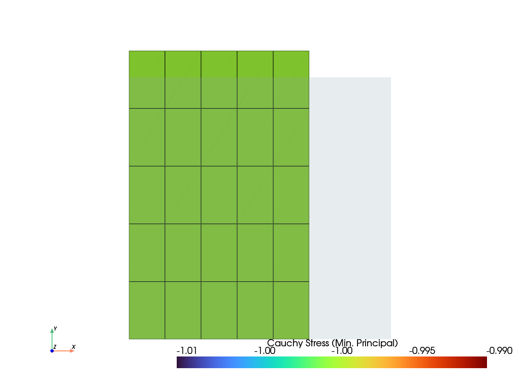
>>> import felupe as fem
>>>
>>> mesh = fem.Rectangle(n=6)
>>> region = fem.RegionQuad(mesh)
>>> field = fem.FieldContainer([fem.FieldAxisymmetric(region, dim=2)])
>>> boundaries = fem.dof.symmetry(field[0])
>>> umat = fem.NeoHooke(mu=1, bulk=2)
>>> solid = fem.SolidBody(umat, field)
>>>
>>> region_pressure = fem.RegionQuadBoundary(
...     mesh=mesh,
...     only_surface=True,  # select only faces on the outline
...     mask=mesh.points[:, 0] == 1,  # select a subset of faces on the surface
...     ensure_3d=True,  # requires True for axisymmetric/plane strain, otherwise False
... )
>>> field_boundary = fem.FieldContainer([fem.FieldAxisymmetric(region_pressure, dim=2)])
>>> pressure = fem.SolidBodyPressure(field=field_boundary)
>>>
>>> table = fem.math.linsteps([0, 1], num=5)
>>> step = fem.Step(
...     items=[solid, pressure], ramp={pressure: 1 * table}, boundaries=boundaries
... )
>>>
>>> job = fem.Job(steps=[step]).evaluate()
>>> solid.plot(
...     "Principal Values of Cauchy Stress", component=2, clim=[-1.01, -0.99]
... ).show()

update(pressure)

class felupe.SolidBodyCauchyStress(field, cauchy_stress=None)

ベースクラス: object

A Cauchy stress boundary on a solid body.

パラメータ:

• field (FieldContainer) -- A field container with fields created on a boundary region.

• stress (ndarray of shape (3, 3, ...) or None, optional) -- The prescribed Cauchy stress components \(\sigma_{ij}\) (default is None). If None, all Cauchy stress components are set to zero.

メモ

\[\delta W_{ext} = \int_{\partial V} \delta \boldsymbol{u} \cdot \boldsymbol{\sigma}\ d\boldsymbol{a} = \int_{\partial V} \delta \boldsymbol{u} \cdot \boldsymbol{\sigma} J \boldsymbol{F}^{-T}\ d\boldsymbol{A}\]

サンプル

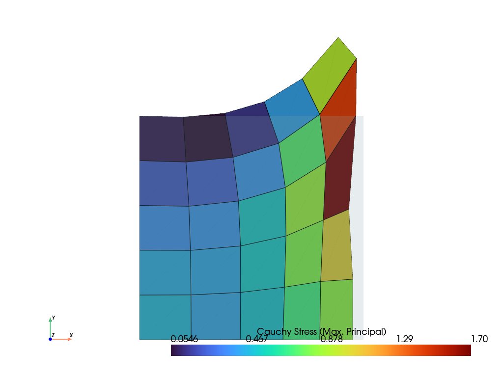
>>> import numpy as np
>>> import felupe as fem
>>>
>>> mesh = fem.Rectangle(n=6)
>>> region = fem.RegionQuad(mesh)
>>> field = fem.FieldContainer([fem.FieldAxisymmetric(region, dim=2)])
>>>
>>> boundaries = {"fixed": fem.Boundary(field[0], fx=0)}
>>> solid = fem.SolidBody(umat=fem.NeoHooke(mu=1, bulk=2), field=field)
>>>
>>> mask = np.logical_and(mesh.x == 1, mesh.y > 0.5)
>>> region_stress = fem.RegionQuadBoundary(
...     mesh=mesh,
...     mask=mask,  # select a subset of faces on the surface
...     ensure_3d=True,  # True for axisymmetric/plane strain
... )
>>> field_boundary = fem.FieldContainer([fem.FieldAxisymmetric(region_stress, dim=2)])
>>> stress = fem.SolidBodyCauchyStress(field=field_boundary)
>>>
>>> table = (
...     fem.math.linsteps([0, 1], num=5, axis=1, axes=9)
...     + fem.math.linsteps([0, 1], num=5, axis=3, axes=9)
... ).reshape(-1, 3, 3)
>>>
>>> step = fem.Step(
...     items=[solid, stress], ramp={stress: 1.0 * table}, boundaries=boundaries
... )
>>> job = fem.Job(steps=[step]).evaluate()
>>> solid.plot("Principal Values of Cauchy Stress").show()

update(cauchy_stress)

class felupe.PointLoad(field, points, values=None, apply_on=0, axisymmetric=False)

ベースクラス: object

A point load with methods for the assembly of sparse vectors/matrices, applied on the n-th field.

パラメータ:

• field (FieldContainer) -- A field container with fields created on a region.

• points (list of int) -- A list with point ids where the values are applied.

• values (float or array_like or None, optional) -- Values at points (default is None). If None, the values are set to zero.

• apply_on (int, optional) -- The n-th field on which the point load is applied (default is 0).

• axisymmetric (bool, optional) -- A flag to multiply the assembled vector and matrix by a scaling factor of \(2 \pi\) (default is False).

サンプル

>>> import felupe as fem
>>>
>>> mesh = fem.mesh.Line(n=3)
>>> element = fem.element.Line()
>>> quadrature = fem.GaussLegendre(order=1, dim=1)
>>>
>>> region = fem.Region(mesh, element, quadrature)
>>> field = fem.FieldContainer([fem.Field(region, dim=1)])
>>>
>>> load = fem.PointLoad(field, [1, 2], values=[[3], [5]])
>>>
>>> vector = load.assemble.vector()
>>> vector.toarray()
array([[0.],
       [3.],
       [5.]])

plot(plotter=None, color='red', scale=0.125, deformed=True, **kwargs)

Plot the point load.

update(values)

class felupe.TrussBody(umat, field, area, statevars=None)

ベースクラス: Solid

A Truss body with methods for the assembly of sparse vectors/matrices.

パラメータ:

• umat (class) -- A class which provides methods for evaluating the gradient and the hessian of the strain energy density function per unit undeformed volume. The function signatures must be dψdλ, ζ_new = umat.gradient([λ, ζ]) for the gradient and d2ψdλdλ = umat.hessian([λ, ζ]) for the hessian of the strain energy density function \(\psi(\lambda)\), where \(\lambda\) is the stretch and \(\zeta\) holds the array of internal state variables.

• field (FieldContainer) -- A field container with one or more fields.

• area (float or ndarray) -- The cross-sectional areas of the trusses.

• statevars (ndarray or None, optional) -- Array of initial internal state variables (default is None).

メモ

For a truss element the stretch is evaluated as given in Eq. (17)

(17)\[\Lambda = \sqrt{\frac{l^2}{L^2}}\]

with the squared undeformed and deformed lengths, denoted in Eqs. (18).

(18)\[\begin{split}l^2 &= \boldsymbol{\Delta x}^T \boldsymbol{\Delta x} \\ L^2 &= \boldsymbol{\Delta X}^T \boldsymbol{\Delta X}\end{split}\]

This enables the Biot strain measure, see Eq. (19).

(19)\[E_{11} = \Lambda - 1\]

The normal force of a truss depends directly on the geometric exactly defined strain measure \(E_{11}\). For the general case of a nonlinear material behaviour the normal force is defined as given in Eq. (20)

(20)\[N = S_{11}(E_{11})~A\]

and the derivative according to Eq. (21).

(21)\[\frac{\partial N}{\partial E_{11}} = \frac{ \partial S_{11}(E_{11}) }{\partial E_{11}}~A\]

For the case of a linear elastic material this reduces to Eqs. (22).

(22)\[\begin{split}S_{11}(E_{11}) &= E~E_{11} \\ N &= EA~E_{11} \\ \frac{\partial N}{\partial E_{11}} &= EA\end{split}\]

The (nonlinear) fixing force column vector may be expressed as a function of the elemental force \(N_k\) and the deformed unit vector \(\boldsymbol{n}_k\), see Eq. (23).

(23)\[\begin{split}\boldsymbol{r}_k = \begin{bmatrix} \boldsymbol{r}_A \\ \boldsymbol{r}_E \end{bmatrix} = N_k \begin{pmatrix} -\boldsymbol{n}_k \\ \phantom{-}\boldsymbol{n}_k \end{pmatrix}\end{split}\]

For a truss the stiffness matrix is divided into four block matrices of the same components but with different signs, see Eq. (24).

(24)\[\begin{split}\boldsymbol{K}_{k~(6,6)} = \begin{bmatrix} \boldsymbol{K}_{AA} & \boldsymbol{K}_{AE}\\ \boldsymbol{K}_{EA} & \boldsymbol{K}_{EE} \end{bmatrix} = \begin{pmatrix} \phantom{-}\boldsymbol{K}_{EE} & -\boldsymbol{K}_{EE}\\ -\boldsymbol{K}_{EE} & \phantom{-}\boldsymbol{K}_{EE} \end{pmatrix}\end{split}\]

A change in the fixing force vector at the end node E w.r.t. a small change of the displacements at node E is defined as the tangent stiffnes EE, see Eq. (25).

(25)\[\begin{split}\boldsymbol{K}_{EE} &= \frac{ \partial \boldsymbol{r}_E}{\partial \boldsymbol{U}_E } \\ \boldsymbol{K}_{EE} &= \frac{A}{L} ~ \frac{ \partial S_{11}(E_{11}) }{\partial E_{11}} \boldsymbol{n} \otimes \boldsymbol{n} + \frac{N}{l} \left( \boldsymbol{1} - \boldsymbol{n} \otimes \boldsymbol{n} \right)\end{split}\]

サンプル

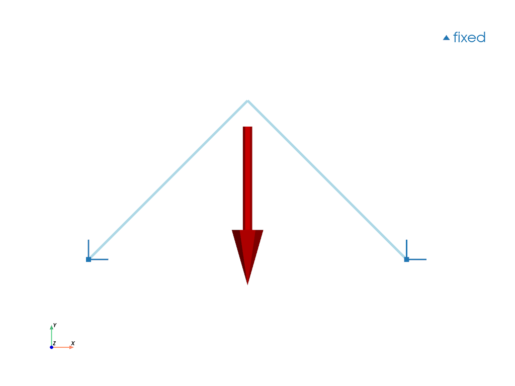
>>> import felupe as fem
>>>
>>> mesh = fem.Mesh(
...     points=[[0, 0], [1, 1], [2.0, 0]],
...     cells=[[0, 1], [1, 2]],
...     cell_type="line",
... )
>>> region = fem.RegionTruss(mesh)
>>> field = fem.Field(region, dim=2).as_container()
>>> boundaries = fem.BoundaryDict(fixed=fem.Boundary(field[0], fy=0))
>>>
>>> umat = fem.LinearElastic1D(E=[1, 1])
>>> truss = fem.TrussBody(umat, field, area=[1, 1])
>>> load = fem.PointLoad(field, points=[1])
>>>
>>> table = fem.math.linsteps([0, 1], num=5, axis=1, axes=2)
>>> ramp = {load: table * -0.1}
>>> step = fem.Step(items=[truss, load], ramp=ramp, boundaries=boundaries)
>>> job = fem.Job(steps=[step]).evaluate()
>>>
>>> mesh.plot(
...     plotter=load.plot(plotter=boundaries.plot(), scale=0.5),
...     line_width=5
... ).show()

class felupe.Step(items, ramp=None, boundaries=None)

ベースクラス: object

A Step with multiple substeps, subsequently depending on the solution of the previous substep.

パラメータ:

• items (list of SolidBody, SolidBodyNearlyIncompressible, SolidBodyPressure, SolidBodyGravity, PointLoad, MultiPointConstraint or MultiPointContact) -- A list of items with methods for the assembly of sparse vectors/matrices.

• ramp (dict, optional) -- A dict with Boundary or item-keys which holds the array of values to ramp (default is None). If None, only one substep is evaluated.

• boundaries (dict of Boundary, optional) -- A dict with Boundary conditions (default is None).

サンプル

>>> import felupe as fem
>>>
>>> mesh = fem.Cube(n=6)
>>> region = fem.RegionHexahedron(mesh)
>>> field = fem.FieldContainer([fem.Field(region, dim=3)])
>>>
>>> boundaries = fem.dof.symmetry(field[0])
>>> boundaries["clamped"] = fem.Boundary(field[0], fx=1, skip=(True, False, False))
>>> boundaries["move"] = fem.Boundary(field[0], fx=1, skip=(False, True, True))
>>>
>>> umat = fem.NeoHooke(mu=1, bulk=2)
>>> solid = fem.SolidBody(umat, field)
>>>
>>> move = fem.math.linsteps([0, 1], num=5)
>>> step = fem.Step(items=[solid], ramp={boundaries["move"]: move}, boundaries=boundaries)
>>>
>>> job = fem.Job(steps=[step]).evaluate()
>>> ax = solid.plot("Principal Values of Cauchy Stress").show()

参考

Job

A job with a list of steps and a method to evaluate them.

CharacteristicCurve

A job with a list of steps and a method to evaluate them. Force-displacement curve data is tracked during evaluation for a given Boundary.

generate(**kwargs)

Yield all generated substeps.

class felupe.Job(steps, callback=<function Job.<lambda>>, plugins=None, **kwargs)

ベースクラス: object

A job with a list of steps and a method to evaluate them.

パラメータ:

• steps (list of Step) -- A list with steps, where each step subsequently depends on the solution of the previous step.

• callback (callable, optional) -- A callable which is called after each completed substep. Function signature must be lambda stepnumber, substepnumber, substep, **kwargs: None, where substep is an instance of NewtonResult. The field container of the completed substep is available as substep.x. Default is callback=lambda stepnumber, substepnumber, substep, **kwargs: None.

• plugins (list or None, optional) -- A list of plugins with hooks to be used during evaluation. Available hooks are before_job, after_job, before_step, after_step and after_substep. Each hook takes the job and the current state as arguments. All hooks are optional. Default is None, which is equivalent to an empty list. Simple callable plugins are dispatched at the after_substep hook.

• **kwargs (dict, optional) -- Optional keyword-arguments for the callback function.

nsteps

The number of steps.

Type:

int

timetrack

A list with times at which the results are written to the XDMF result file.

Type:

list of int

fnorms

List with norms of the objective function for each completed substep of each step. See also class:~felupe.tools.NewtonResult.

Type:

list of list of float

サンプル

>>> import felupe as fem
>>>
>>> mesh = fem.Cube(n=6)
>>> region = fem.RegionHexahedron(mesh)
>>> field = fem.FieldContainer([fem.Field(region, dim=3)])
>>>
>>> boundaries = fem.dof.symmetry(field[0])
>>> boundaries["clamped"] = fem.Boundary(field[0], fx=1, skip=(True, False, False))
>>> boundaries["move"] = fem.Boundary(field[0], fx=1, skip=(False, True, True))
>>>
>>> umat = fem.NeoHooke(mu=1, bulk=2)
>>> solid = fem.SolidBody(umat, field)
>>>
>>> move = fem.math.linsteps([0, 1], num=5)
>>> step = fem.Step(items=[solid], ramp={boundaries["move"]: move}, boundaries=boundaries)
>>>
>>> job = fem.Job(steps=[step]).evaluate()
>>> solid.plot("Principal Values of Cauchy Stress").show()

参考

Step

A Step with multiple substeps, subsequently depending on the solution of the previous substep.

CharacteristicCurve

A job with a list of steps and a method to evaluate them. Force-displacement curve data is tracked during evaluation for a given Boundary.

tools.NewtonResult

A data class which represents the result found by Newton's method.

evaluate(filename=None, mesh=None, point_data=None, cell_data=None, point_data_default=True, cell_data_default=True, verbose=None, parallel=False, tqdm='tqdm', **kwargs)

Evaluate the steps.

パラメータ:

• filename (str or None, optional) -- The filename of the XDMF result file. Must include the file extension my_result.xdmf. If None, no result file is written during evaluation. Default is None.

• mesh (Mesh or None, optional) -- A mesh which is used for the XDMF time series writer. If None, it is taken from the field of the first item of the first step if no keyword argument x0 is given. If None and x0=field, the mesh is taken from the x0 field container. Default is None.

• point_data (dict or None, optional) -- Additional dict of point-data for the meshio XDMF time series writer.

• cell_data (dict or None, optional) -- Additional dict of cell-data for the meshio XDMF time series writer.

• point_data_default (bool, optional) -- Flag to write default point-data to the XDMF result file. This includes "Displacement". Default is True.

• cell_data_default (bool, optional) -- Flag to write default cell-data to the XDMF result file. This includes "Principal Values of Logarithmic Strain", "Logarithmic Strain" and "Deformation Gradient". Default is True.

• verbose (bool or int or None, optional) -- Verbosity level to control how messages are printed during evaluation. If 1 or True and tqdm is installed, a progress bar is shown. If tqdm is missing or verbose is 2, more detailed text-based messages are printed. Default is None. If None, verbosity is set to True. If None and the environmental variable FELUPE_VERBOSE is set and its value is not true, then logging is turned off.

• parallel (bool, optional) -- Flag to use a threaded version of numpy.einsum() during assembly. Requires einsumt. This may add additional overhead to small-sized problems. Default is False.

• tqdm (str, optional) -- If verbose is True, choose a backend for tqdm ("tqdm", "auto" or "notebook". Default is "tqdm".

• **kwargs (dict) -- Optional keyword arguments for generate(). If parallel=True, it is added as kwargs["parallel"] = True to the dict of additional keyword arguments. If x0 is present in kwargs.keys(), it is used as the mesh for the XDMF time series writer.

戻り値:

The job object.

戻り値の型:

Job

メモ

Requires meshio and h5py if filename is not None. Also requires tqdm for an interactive progress bar if verbose=True.

参考

Step

A Step with multiple substeps, subsequently depending on the solution of the previous substep.

CharacteristicCurve

A job with a list of steps and a method to evaluate them. Force-displacement curve data is tracked during evaluation for a given Boundary condition.

tools.NewtonResult

A data class which represents the result found by Newton's method.

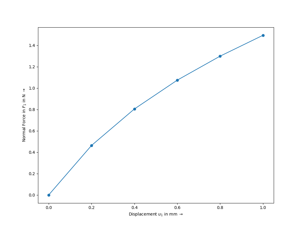
class felupe.CharacteristicCurve(steps, boundary, items=None, callback=<function CharacteristicCurve.<lambda>>, **kwargs)

ベースクラス: Job

A job with a list of steps and a method to evaluate them. Force-displacement curve data is tracked during evaluation for a given Boundary by a built-in callback.

パラメータ:

• steps (list of Step) -- A list with steps, where each step subsequently depends on the solution of the previous step.

• items (list of SolidBody, SolidBodyNearlyIncompressible, SolidBodyPressure, SolidBodyGravity, PointLoad, MultiPointConstraint, MultiPointContact or None, optional) -- A list of items with methods for the assembly of sparse vectors/matrices which are used to evaluate the sum of reaction forces. If None, the total reaction forces from the NewtonResult of the substep are used.

• callback (callable, optional) -- A callable which is called after each completed substep. Function signature must be lambda stepnumber, substepnumber, substep, **kwargs: None, where substep is an instance of NewtonResult. The field container of the completed substep is available as substep.x. Default is callback=lambda stepnumber, substepnumber, substep, **kwargs: None.

• **kwargs (dict, optional) -- Optional keyword-arguments for the callback function.

サンプル

>>> import felupe as fem
>>>
>>> mesh = fem.Cube(n=6)
>>> region = fem.RegionHexahedron(mesh)
>>> field = fem.FieldContainer([fem.Field(region, dim=3)])
>>>
>>> boundaries = dict()
>>> boundaries["fixed"] = fem.Boundary(field[0], fx=0, skip=(False, False, False))
>>> boundaries["clamped"] = fem.Boundary(field[0], fx=1, skip=(True, False, False))
>>> boundaries["move"] = fem.Boundary(field[0], fx=1, skip=(False, True, True))
>>>
>>> umat = fem.NeoHooke(mu=1, bulk=2)
>>> solid = fem.SolidBody(umat, field)
>>>
>>> move = fem.math.linsteps([0, 1], num=5)
>>> step = fem.Step(items=[solid], ramp={boundaries["move"]: move}, boundaries=boundaries)
>>>
>>> job = fem.CharacteristicCurve(steps=[step], boundary=boundaries["move"]).evaluate()
>>> solid.plot("Principal Values of Cauchy Stress").show()

>>> fig, ax = job.plot(
...    xlabel=r"Displacement $u_1$ in mm $\rightarrow$",
...    ylabel=r"Normal Force in $F_1$ in N $\rightarrow$",
...    marker="o",
... )

参考

Step

A Step with multiple substeps, subsequently depending on the solution of the previous substep.

Job

A job with a list of steps and a method to evaluate them.

tools.NewtonResult

A data class which represents the result found by Newton's method.

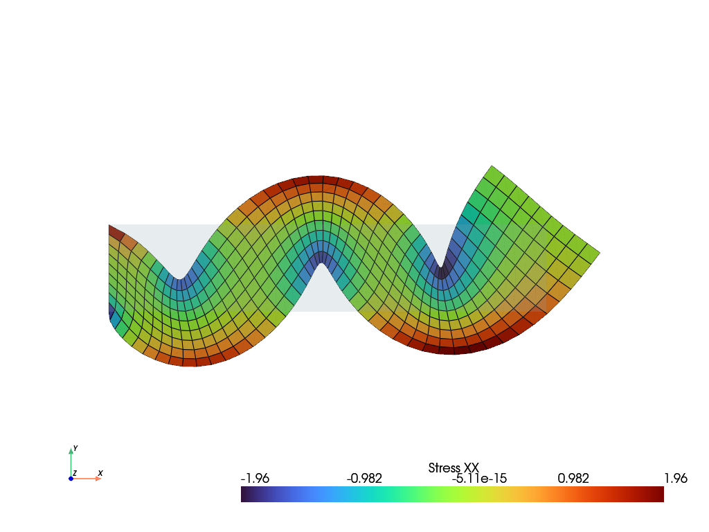
class felupe.FreeVibration(items, boundaries=None)

ベースクラス: object

A Free-Vibration Step/Job.

パラメータ:

• items (list of SolidBody or SolidBodyNearlyIncompressible) -- A list of items with methods for the assembly of sparse stiffness and mass matrices.

• boundaries (dict of Boundary, optional) -- A dict with Boundary conditions (default is None).

メモ

注釈

Boundary conditions with non-zero values are not supported.

サンプル

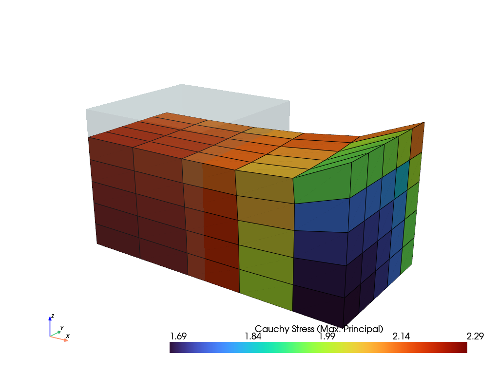
>>> import felupe as fem
>>> import numpy as np
>>>
>>> mesh = fem.Rectangle(b=(5, 1), n=(50, 10))
>>> region = fem.RegionQuad(mesh)
>>> field = fem.FieldContainer([fem.FieldPlaneStrain(region, dim=2)])
>>>
>>> boundaries = dict(left=fem.Boundary(field[0], fx=0))
>>> solid = fem.SolidBody(fem.LinearElastic(E=2.5, nu=0.25), field, density=1.0)
>>> modal = fem.FreeVibration(items=[solid], boundaries=boundaries).evaluate()
>>>
>>> eigenvector, frequency = modal.extract(n=4, inplace=True)
>>> solid.plot("Stress", component=0).show()

evaluate(x0=None, solver=<function eigsh>, parallel=False, **kwargs)

extract(n=0, x0=None, inplace=True)

class felupe.AnimationWriterPlugin(items, filename='animation.gif', framerate=5, quality=5, zoom_camera=1.0, reset_camera=True, show_text=True, take_screenshots=False, **kwargs)

ベースクラス: Plugin

A job plugin to write an animation file during job evaluation.

パラメータ:

• items (list) -- The items to plot.

• filename (str or None, optional) -- The filename of the animation file. Default is "animation.gif". Supported formats are GIF and MP4 (or any other format supported by PyVista). If None, no animation file will be written. Default is "animation.gif".

• framerate (int, optional) -- The framerate of the animation. Default is 5.

• quality (int, optional) -- The quality of the movie. Default is 5. This is only used for movie formats, not for GIFs.

• zoom_camera (float, optional) -- The zoom factor for the camera. Default is 1.0.

• reset_camera (bool, optional) -- Whether to reset the camera before each frame. Default is True.

• show_text (bool, optional) -- Whether to show text on the plot. Default is True.

• take_screenshots (bool or None, optional) -- Whether to take screenshots for all substeps per step. If True, the screenshots will be saved in the "figures" folder. Default is False.

• **kwargs (dict, optional) -- Additional keyword arguments to pass to the plot method of the items.

メモ

This plugin should be used with off_screen=True. While it is possible to show the plotter during the job evaluation, it may flicker.

サンプル

>>> import felupe as fem
>>>
>>> mesh = fem.Cube(n=6)
>>> region = fem.RegionHexahedron(mesh)
>>> field = fem.FieldContainer([fem.Field(region, dim=3)])
>>>
>>> boundaries = fem.dof.uniaxial(
...     field, clamped=True, return_loadcase=False
... )
>>> umat = fem.NeoHooke(mu=1, bulk=2)
>>> solid = fem.SolidBody(umat=umat, field=field)
>>>
>>> move = fem.math.linsteps([0, 1, 0], num=5)
>>> ramp = {boundaries["move"]: move}
>>> step = fem.Step(items=[solid], ramp=ramp, boundaries=boundaries)
>>>
>>> animation = fem.AnimationWriterPlugin(
...     items=[field],
...     filename="animation.gif",
...     name="Principal Values of Logarithmic Strain",
... )
>>> job = fem.Job(steps=[step], plugins=[animation])
>>> job.evaluate()

参考

felupe.Job

A job with a list of steps and a method to evaluate them.

after_iteration(context, state)

This method is called after a Newton-Raphson iteration.

パラメータ:

• context (felupe.Context) -- The context object.

• state (felupe.IterationState) -- The state of the iteration.

after_job(context, state)

This method is called after the evaluation of a job.

パラメータ:

• context (felupe.Context) -- The context object.

• state (felupe.JobState) -- The state of the job.

after_substep(context, state)

This method is called after a substep.

パラメータ:

• context (felupe.Context) -- The context object.

• state (felupe.IterationState) -- The state of the iteration.

before_job(context, state)

This method is called before the evaluation of a job.

パラメータ:

• context (felupe.Context) -- The context object.

• state (felupe.JobState) -- The state of the job.

class felupe.CharacteristicCurvePlugin(boundary, items=None)

ベースクラス: Plugin

A job plugin to record a characteristic curve. Force-displacement curve data is tracked during evaluation for a given Boundary.

パラメータ:

• boundary (felupe.Boundary) -- The boundary condition for which to record the characteristic curve.

• items (list of SolidBody, SolidBodyNearlyIncompressible, SolidBodyPressure, SolidBodyGravity, PointLoad, MultiPointConstraint, MultiPointContact or None, optional) -- A list of items with methods for the assembly of sparse vectors/matrices which are used to evaluate the sum of reaction forces. If None, the total reaction forces from the NewtonResult of the substep are used.

サンプル

>>> import felupe as fem
>>>
>>> mesh = fem.Cube(n=6)
>>> region = fem.RegionHexahedron(mesh)
>>> field = fem.FieldContainer([fem.Field(region, dim=3)])
>>>
>>> boundaries = dict()
>>> boundaries["fixed"] = fem.Boundary(field[0], fx=0, skip=(False, False, False))
>>> boundaries["clamped"] = fem.Boundary(field[0], fx=1, skip=(True, False, False))
>>> boundaries["move"] = fem.Boundary(field[0], fx=1, skip=(False, True, True))
>>>
>>> umat = fem.NeoHooke(mu=1, bulk=2)
>>> solid = fem.SolidBody(umat, field)
>>>
>>> move = fem.math.linsteps([0, 1], num=5)
>>> step = fem.Step(items=[solid], ramp={boundaries["move"]: move}, boundaries=boundaries)
>>>
>>> curve = fem.CharacteristicCurvePlugin(boundary=boundaries["move"])
>>> job = fem.Job(steps=[step], plugins=[curve]).evaluate()
>>> solid.plot("Principal Values of Cauchy Stress").show()

>>> fig, ax = curve.plot(
...    xlabel=r"Displacement $u_1$ in mm $\rightarrow$",
...    ylabel=r"Normal Force in $F_1$ in N $\rightarrow$",
...    marker="o",
... )

参考

felupe.Job

A job with a list of steps and a method to evaluate them.

after_substep(context, state)

This method is called after a substep.

パラメータ:

• context (felupe.Context) -- The context object.

• state (felupe.IterationState) -- The state of the iteration.

plot(x=None, y=None, xaxis=0, yaxis=0, xlabel=None, ylabel=None, xscale=1.0, yscale=1.0, xoffset=0.0, yoffset=0.0, gradient=False, swapaxes=False, ax=None, items=None, **kwargs)

Plot force-displacement characteristic curves on a pre-evaluated job, tracked on a given Boundary.

パラメータ:

• x (list of ndarray or None, optional) -- A list with arrays of displacement data. If None, the displacement is taken from the first field of the field container from each completed substep. The displacement data is then taken from the first point of the tracked Boundary. Default is None.

• y (list of ndarray or None, optional) -- A list with arrays of reaction force data. If None, the force is taken from the NewtonResult of each completed substep. Default is None.

• xaxis (int, optional) -- The axis for the displacement data (default is 0).

• yaxis (int, optional) -- The axis for the reaction force data (default is 0).

• xlabel (str or None, optional) -- The label of the x-axis (default is None).

• ylabel (str or None, optional) -- The label of the y-axis (default is None).

• xscale (float, optional) -- A scaling factor for the displacement data (default is 1.0).

• yscale (float, optional) -- A scaling factor the reaction force data (default is 1.0).

• xoffset (float, optional) -- An offset for the displacement data (default is 0.0).

• yoffset (float, optional) -- An offset for the reaction force data (default is 0.0).

• gradient (bool, optional) -- A flag to plot the gradient of the y-data. Uses numpy.gradient(edge_order=2). The gradient data is set to np.nan for absolute values greater than the mean value plus two times the standard deviation. Default is False.

• swapaxes (bool, optional) -- A flag to flip the plot (x, y) to (y, x). Also changes the labels.

• ax (matplotlib.axes.Axes) -- An axes object where the plot is placed in.

• items (slice, ndarray or None) -- Indices or a range of data points to plot. If None, all data points are plotted (default is None).

• **kwargs (dict) -- Additional keyword arguments for plotting in ax.plot(**kwags).

戻り値:

• fig (matplotlib.figure.Figure) -- The figure object where the plot is placed in.

• ax (matplotlib.axes.Axes) -- The axes object where the plot is placed in.

class felupe.ProgressPlugin(verbose=None, tqdm='tqdm')

ベースクラス: Plugin

A job plugin to output the progress of a job evaluation in the terminal.

パラメータ:

• verbose (bool or int or None, optional) -- Verbosity level to control how messages are printed during evaluation. If 1 or True and tqdm is installed, a progress bar is shown. If tqdm is missing or verbose is 2, more detailed text-based messages are printed. Default is None. If None, verbosity is set to True. If None and the environmental variable FELUPE_VERBOSE is set and its value is not true, then logging is turned off.

• tqdm (str, optional) -- If verbose is True, choose a backend for tqdm ("tqdm", "auto" or "notebook". Default is "tqdm".

メモ

Requires tqdm for an interactive progress bar if verbose=True.

参考

felupe.Job

A job with a list of steps and a method to evaluate them.

after_iteration(context, state)

This method is called after a Newton-Raphson iteration.

パラメータ:

• context (felupe.Context) -- The context object.

• state (felupe.IterationState) -- The state of the iteration.

after_job(context, state)

This method is called after the evaluation of a job.

パラメータ:

• context (felupe.Context) -- The context object.

• state (felupe.JobState) -- The state of the job.

after_linear_solve(context, state)

This method is called after the linear solver inside a Newton-Raphson iteration.

パラメータ:

• context (felupe.Context) -- The context object.

• state (felupe.IterationState) -- The state of the iteration.

after_newton(context, state)

This method is called after the Newton-Raphson solver.

パラメータ:

• context (felupe.Context) -- The context object.

• state (felupe.IterationState) -- The state of the iteration.

after_substep(context, state)

This method is called after a substep.

パラメータ:

• context (felupe.Context) -- The context object.

• state (felupe.IterationState) -- The state of the iteration.

before_job(context, state)

This method is called before the evaluation of a job.

パラメータ:

• context (felupe.Context) -- The context object.

• state (felupe.JobState) -- The state of the job.

before_linear_solve(context, state)

This method is called before the linear solver inside a Newton-Raphson iteration.

パラメータ:

• context (felupe.Context) -- The context object.

• state (felupe.IterationState) -- The state of the iteration.

before_newton(context, state)

This method is called before the Newton-Raphson solver.

パラメータ:

• context (felupe.Context) -- The context object.

• state (felupe.IterationState) -- The state of the iteration.

before_step(context, state)

This method is called before a step.

パラメータ:

• context (felupe.Context) -- The context object.

• state (felupe.JobState) -- The state of the job.

configure(verbose, tqdm)

Configure the plugin. This can be called after initialization to change the parameters.

class felupe.XDMFWriterPlugin(filename=None, mesh=None, point_data=None, cell_data=None, point_data_default=False, cell_data_default=False, kwargs=None)

ベースクラス: Plugin

A job plugin to write XDMF files during job evaluation.

メモ

Requires h5py.

参考

felupe.Job

A job with a list of steps and a method to evaluate them.

after_iteration(context, state)

This method is called after a Newton-Raphson iteration.

パラメータ:

• context (felupe.Context) -- The context object.

• state (felupe.IterationState) -- The state of the iteration.

after_job(context, state)

This method is called after the evaluation of a job.

パラメータ:

• context (felupe.Context) -- The context object.

• state (felupe.JobState) -- The state of the job.

after_substep(context, state)

This method is called after a substep.

パラメータ:

• context (felupe.Context) -- The context object.

• state (felupe.IterationState) -- The state of the iteration.

before_job(context, state)

This method is called before the evaluation of a job.

パラメータ:

• context (felupe.Context) -- The context object.

• state (felupe.JobState) -- The state of the job.

configure(filename, mesh, point_data, cell_data, point_data_default, cell_data_default, kwargs)

class felupe.Plugin

ベースクラス: object

Base class for plugins.

メモ

All methods (hooks) are optional and will be called at the appropriate time during the simulation. The context and state objects are passed to each method, allowing a plugin to access and / or modify a simulation as needed.

The Context object holds information about the current job, step or substep. state depends on the method and can be used to access the current state, i.e. JobState or IterationState.

注釈

All methods are optional.

参考

felupe.Job

A job with a list of steps and a method to evaluate them.

felupe.EventDispatcher

A class to dispatch events to plugins during evaluation.

felupe.Context

A class to keep track of the context of a Job during evaluation.

felupe.JobState

A class to keep track of the state of a Job during evaluation.

felupe.IterationState

A class to keep track of the state of an iteration.

after_iteration(context, state)

This method is called after a Newton-Raphson iteration.

パラメータ:

• context (felupe.Context) -- The context object.

• state (felupe.IterationState) -- The state of the iteration.

after_job(context, state)

This method is called after the evaluation of a job.

パラメータ:

• context (felupe.Context) -- The context object.

• state (felupe.JobState) -- The state of the job.

after_linear_solve(context, state)

This method is called after the linear solver inside a Newton-Raphson iteration.

パラメータ:

• context (felupe.Context) -- The context object.

• state (felupe.IterationState) -- The state of the iteration.

after_newton(context, state)

This method is called after the Newton-Raphson solver.

パラメータ:

• context (felupe.Context) -- The context object.

• state (felupe.IterationState) -- The state of the iteration.

after_step(context, state)

This method is called after a step.

パラメータ:

• context (felupe.Context) -- The context object.

• state (felupe.JobState) -- The state of the job.

after_substep(context, state)

This method is called after a substep.

パラメータ:

• context (felupe.Context) -- The context object.

• state (felupe.IterationState) -- The state of the iteration.

before_iteration(context, state)

This method is called before a Newton-Raphson iteration.

パラメータ:

• context (felupe.Context) -- The context object.

• state (felupe.IterationState) -- The state of the iteration.

before_job(context, state)

This method is called before the evaluation of a job.

パラメータ:

• context (felupe.Context) -- The context object.

• state (felupe.JobState) -- The state of the job.

before_linear_solve(context, state)

This method is called before the linear solver inside a Newton-Raphson iteration.

パラメータ:

• context (felupe.Context) -- The context object.

• state (felupe.IterationState) -- The state of the iteration.

before_newton(context, state)

This method is called before the Newton-Raphson solver.

パラメータ:

• context (felupe.Context) -- The context object.

• state (felupe.IterationState) -- The state of the iteration.

before_step(context, state)

This method is called before a step.

パラメータ:

• context (felupe.Context) -- The context object.

• state (felupe.JobState) -- The state of the job.

class felupe.EventDispatcher(plugins=None)

ベースクラス: object

A class to dispatch events to plugins during evaluation.

パラメータ:

plugins (list or None, optional) -- The list of plugins.

add_plugin(plugin)

Add a plugin to the dispatcher and reconfigure it.

configure(plugins)

Configure the dispatcher with the given plugins and return a dict with hooks as keys.

trigger(hook, context, state)

Trigger a hook with context and current state to all registered functions.

class felupe.Context(job=None, step=None, substep=None)

ベースクラス: object

A class to keep track of the context of a Job during evaluation.

パラメータ:

• job (felupe.Job or None, optional) -- The job object.

• step (felupe.Step or None, optional) -- The step object.

• substep (felupe.FieldContainer or None, optional) -- The field container object.

class felupe.JobState(stepnumber=None, substepnumber=None, time=None)

ベースクラス: object

A class to keep track of the state of a Job during evaluation.

class felupe.IterationState(iteration=None, fnorm=None, xnorm=None, success=None, tol=None, error=None)

ベースクラス: object

A class to keep track of the state of an iteration during evaluation.

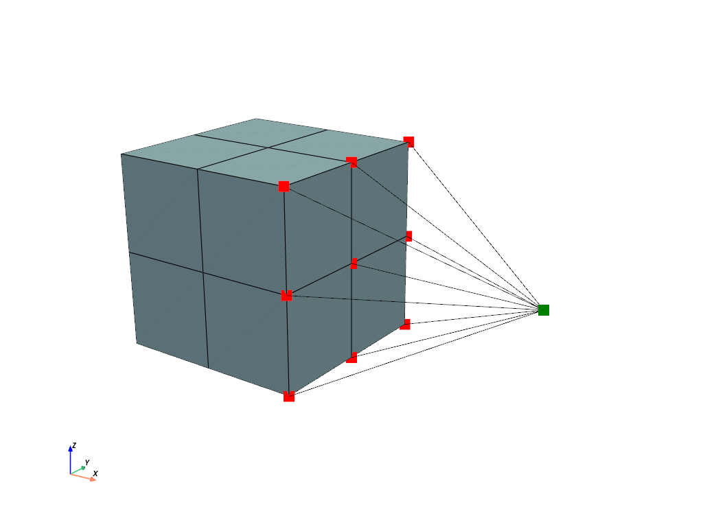
class felupe.MultiPointConstraint(field, points, centerpoint, skip=(False, False, False), multiplier=1000.0)

A Multi-point-constraint which connects a center-point to a list of points.

パラメータ:

• field (FieldContainer) -- A field container with the displacement field as first field.

• points ((n,) ndarray) -- An array with indices of points to be connected to the center-point.

• centerpoint (int) -- The index of the centerpoint.

• skip (3-tuple of bool, optional) -- A tuple with boolean values for each axis to skip. If True, the respective axis is not connected. Default is (False, False, False).

• multiplier (float, optional) -- A multiplier to penalize the relative displacements between the center-point and the points. Default is 1e3.

メモ

A MultiPointConstraint is supported as an item in a Step. It provides the assemble-methods MultiPointConstraint.assemble.vector() and MultiPointConstraint.assemble.matrix().

注釈

Rotational degrees-of-freedom of the center-point are not connected to the points.

サンプル

This example shows how to use a MultiPointConstraint. An additional center-point is added to a mesh.

>>> import numpy as np
>>> import felupe as fem
>>>
>>> mesh = fem.Cube(n=3)
>>> mesh.add_points([2.0, 0.5, 0.5])
>>>
>>> region = fem.RegionHexahedron(mesh)
>>> displacement = fem.Field(region, dim=3)
>>> field = fem.FieldContainer([displacement])
>>>
>>> umat = fem.NeoHooke(mu=1.0, bulk=2.0)
>>> solid = fem.SolidBody(umat=umat, field=field)

A MultiPointConstraint defines the multi-point constraint which connects the displacement degrees of freedom of the center-point with the dofs of points located at \(x=1\).

>>> import pyvista as pv
>>>
>>> mpc = fem.MultiPointConstraint(
...     field=field,
...     points=np.arange(mesh.npoints)[mesh.x == 1],
...     centerpoint=-1,
... )
>>>
>>> plotter = pv.Plotter()
>>> actor_1 = plotter.add_points(
...     mesh.points[mpc.points],
...     point_size=16,
...     color="red",
... )
>>> actor_2 = plotter.add_points(
...     mesh.points[[mpc.centerpoint]],
...     point_size=16,
...     color="green",
... )
>>> mesh.plot(plotter=mpc.plot(plotter=plotter)).show()

The mesh is fixed on the left end face and a ramped PointLoad is applied on the center-point of the MultiPointConstraint. All items are added to a Step and a Job is evaluated.

>>> boundaries = {"fixed": fem.Boundary(displacement, fx=0)}
>>> load = fem.PointLoad(field, points=[-1])
>>> table = fem.math.linsteps([0, 1], num=5, axis=0, axes=3)
>>>
>>> step = fem.Step(
...     [solid, mpc, load], boundaries=boundaries, ramp={load: table}
... )
>>> job = fem.Job([step]).evaluate()

A view on the deformed mesh including the MultiPointConstraint is plotted.

>>> plotter = pv.Plotter()
>>>
>>> actor_1 = plotter.add_points(
...     mesh.points[mpc.points] + displacement.values[mpc.points],
...     point_size=16,
...     color="red",
... )
>>> actor_2 = plotter.add_points(
...     mesh.points[[mpc.centerpoint]] + displacement.values[[mpc.centerpoint]],
...     point_size=16,
...     color="green",
... )
>>> field.plot("Displacement", component=None, plotter=mpc.plot(plotter=plotter)).show()

参考

felupe.MultiPointContact

A frictionless point-to-rigid (wall) contact.

plot(plotter=None, color='black', deformed=True, **kwargs)

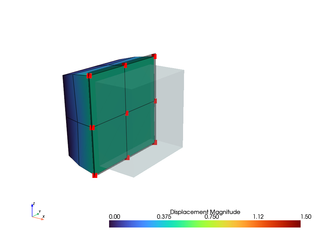
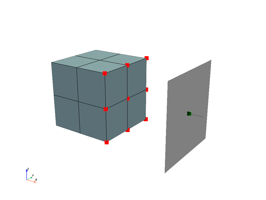
class felupe.MultiPointContact(field, points, centerpoint, skip=(False, False, False), multiplier=1000000.0)

A frictionless point-to-rigid (wall) contact which connects a center-point to a list of points.

パラメータ:

• field (FieldContainer) -- A field container with the displacement field as first field.

• points ((n,) ndarray) -- An array with indices of points to be connected to the center-point.

• centerpoint (int) -- The index of the centerpoint.

• skip (3-tuple of bool, optional) -- A tuple with boolean values for each axis to skip. If True, the respective axis is not connected. Default is (False, False, False).

• multiplier (float, optional) -- A multiplier to penalize the relative displacements between the center-point and the points in contact. Default is 1e6.

メモ

A MultiPointContact is supported as an item in a Step. It provides the assemble-methods MultiPointContact.assemble.vector() and MultiPointContact.assemble.matrix().

サンプル

This example shows how to use a MultiPointContact. An additional center-point is added to a mesh.

>>> import numpy as np
>>> import felupe as fem
>>>
>>> mesh = fem.Cube(n=3)
>>> mesh.add_points([2.0, 0.5, 0.5])
>>>
>>> # prevent the field-values at the center-point to be treated as dof0
>>> mesh.points_without_cells = mesh.points_without_cells[:-1]
>>>
>>> region = fem.RegionHexahedron(mesh)
>>> displacement = fem.Field(region, dim=3)
>>> field = fem.FieldContainer([displacement])
>>>
>>> umat = fem.NeoHooke(mu=1.0, bulk=2.0)
>>> solid = fem.SolidBody(umat=umat, field=field)

A MultiPointContact defines the multi-point contact which connects the displacement degrees of freedom of the center-point with the dofs of points located at \(x=1\) if they are in contact. Only the \(x\)-component is considered in this example.

>>> import pyvista as pv
>>>
>>> contact = fem.MultiPointContact(
...     field=field,
...     points=np.arange(mesh.npoints)[mesh.x == 1],
...     centerpoint=-1,
...     skip=(False, True, True)
... )
>>>
>>> plotter = pv.Plotter()
>>> actor_1 = plotter.add_points(
...     mesh.points[contact.points],
...     point_size=16,
...     color="red",
... )
>>> actor_2 = plotter.add_points(
...     mesh.points[[contact.centerpoint]],
...     point_size=16,
...     color="green",
... )
>>> mesh.plot(plotter=contact.plot(plotter=plotter)).show()

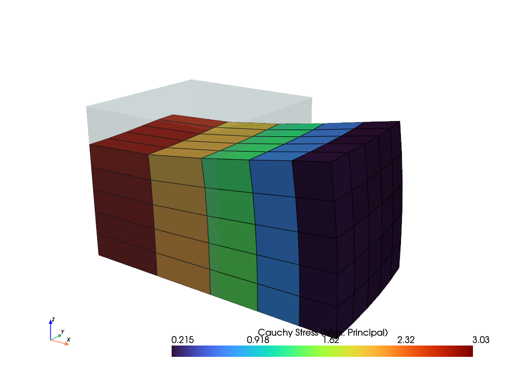
The mesh is fixed on the left end face and a ramped Boundary is applied on the center-point of the MultiPointContact. All items are added to a Step and a Job is evaluated.

>>> boundaries = {
...     "fixed": fem.Boundary(displacement, fx=0),
...     "control": fem.Boundary(displacement, fx=2, skip=(1, 0, 0)),
...     "move": fem.Boundary(displacement, fx=2, skip=(0, 1, 1)),
... }
>>> table = fem.math.linsteps([0, -1, -1.5], num=5)
>>> step = fem.Step(
...     [solid, contact],
...     boundaries=boundaries,
...     ramp={boundaries["move"]: table},
... )
>>> job = fem.Job([step]).evaluate()

A view on the deformed mesh including the MultiPointContact is plotted.

>>> plotter = pv.Plotter()
>>>
>>> actor_1 = plotter.add_points(
...     mesh.points[contact.points] + displacement.values[contact.points],
...     point_size=16,
...     color="red",
... )
>>> actor_2 = plotter.add_points(
...     mesh.points[[contact.centerpoint]] + displacement.values[[contact.centerpoint]],
...     point_size=16,
...     color="green",
... )
>>> field.plot("Displacement", component=None, plotter=contact.plot(plotter=plotter)).show()

参考

felupe.MultiPointConstraint

A Multi-point-constraint which connects a center-point to a list of points.

plot(plotter=None, offset=0, show_edges=True, color='black', opacity=0.5, deformed=True, **kwargs)

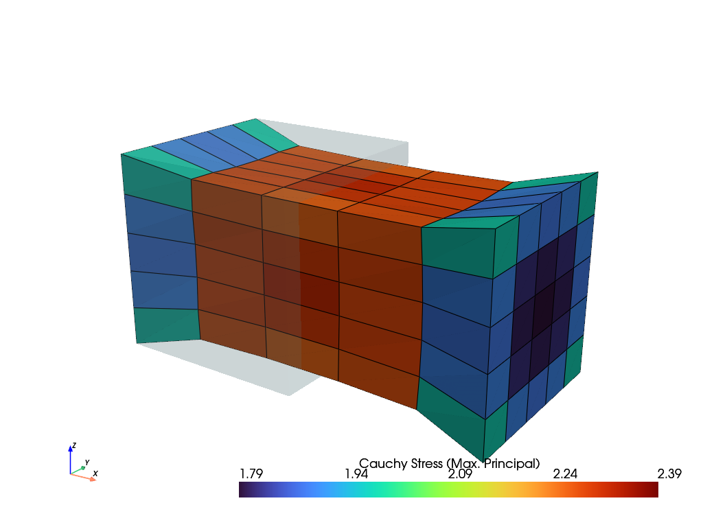
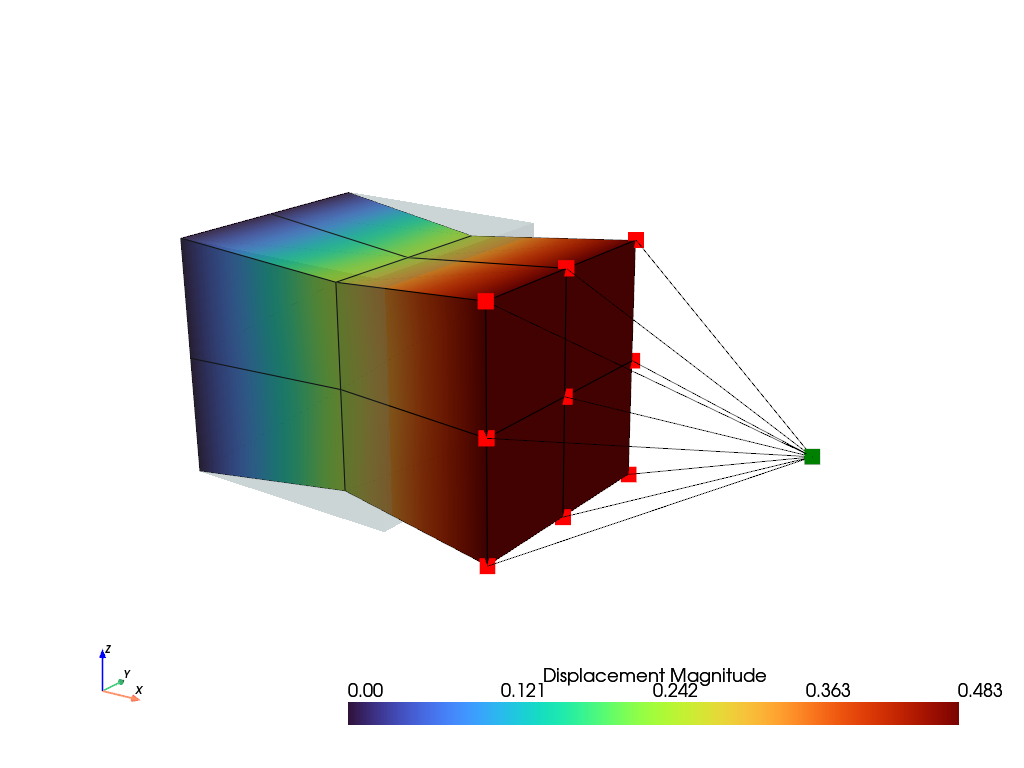
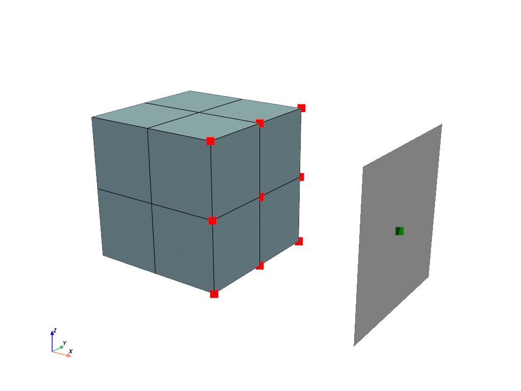
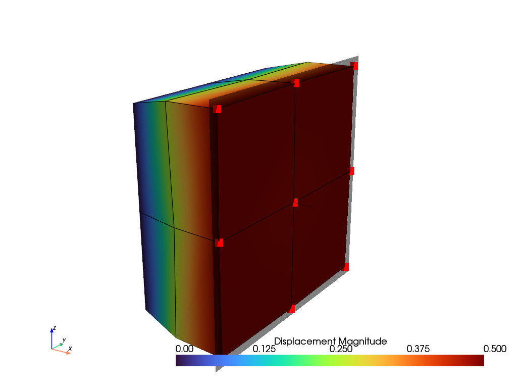
class felupe.ContactRigidPlane(field, points, centerpoint, normal, friction=0.0, multiplier=1.0, multiplier_tangential=0.1, items=None)

A node-to-surface contact, where the surface is given by a rigid plane.

パラメータ:

• field (FieldContainer) -- A field container with the displacement field as first field.

• points ((n,) ndarray) -- An array with indices of points to be connected to the center-point.

• centerpoint (int) -- The index of the centerpoint.

• normal (ndarray) -- The outward plane normal vector.

• friction (float, optional) -- Coulomb friction coefficient \(\mu\). Default is 0.0.

• multiplier (float, optional) -- A scale factor for the multiplier to penalize the relative displacements between the center-point and the points in contact. Default is 1.0. The final multiplier is scaled times a base multiplier, based on the mean normal stiffness, if items are given.

• multiplier_tangential (float or None, optional) -- A scale factor for the multiplier to penalize the relative tangential displacements between the center-point and the points in contact. Default is 0.1. The final multiplier is scaled times a base multiplier, based on the mean tangential stiffness, if items are given.

• items (list or None, optional) -- A list of items to be considered for the evaluation of the mean stiffness-based multipliers. If None, the multipliers are not based on the mean stiffness. Default is None.

メモ

A ContactRigidPlane is supported as an item in a Step.

注釈

The contact formulation is based on a penalty method. The multiplier should be chosen sufficiently large to enforce the contact constraints, but not too large to cause numerical issues. Best practice is to provide items, which are connected to the contact points. This will enable mean stiffness-based multipliers.

The contact activation is based on the gap between the center-point and the points in potential contact. The gap is evaluated in the deformed configuration in the direction of the plane normal. If the gap is negative, the contact is active, see Eq. (26).

(26)\[ \begin{align}\begin{aligned}\Delta \boldsymbol{x} &= \boldsymbol{x} - \boldsymbol{x}_c\\g &= \Delta \boldsymbol{x} \cdot \boldsymbol{n}\\g &\lt 0 \quad \text{(contact active)}\end{aligned}\end{align} \]

The contact normal force and tangent stiffness matrix are evaluated as a penalty contribution proportional to the gap, see Eq. (27).

(27)\[ \begin{align}\begin{aligned}\boldsymbol{f} &= \lambda\ g\ \boldsymbol{n}\\\boldsymbol{P}_n &= \boldsymbol{n} \otimes \boldsymbol{n}\\\boldsymbol{K}_n &= \lambda\ \boldsymbol{P}_n\end{aligned}\end{align} \]

The tangential contact friction forces are evaluated according to a Coulomb friction law, see Eq. (28) and Eq. (29).

(28)\[ \begin{align}\begin{aligned}\Delta \boldsymbol{x}_t &= \Delta \boldsymbol{x} - \Delta \boldsymbol{x}^{ref}\\\boldsymbol{P}_t &= \boldsymbol{1} - \boldsymbol{P}_n\\\boldsymbol{f}_t^{trial} &= \lambda \boldsymbol{P}_t\ \Delta \boldsymbol{x}_t\\f_t^{limit} &= \mu |\boldsymbol{f}_n|\end{aligned}\end{align} \]

(29)\[\begin{split}\text{state} = \begin{cases} |\boldsymbol{f}_t^{trial}| \leq f_t^{limit} & \text{stick} \\ \text{else} & \text{slip} \end{cases}\end{split}\]

In case of sticking contact, the tangential forces are equal to the trial forces, see Eq. (30).

(30)\[ \begin{align}\begin{aligned}\boldsymbol{f}_t &= \boldsymbol{f}_t^{trial}\\\boldsymbol{K}_t &= \lambda\ \boldsymbol{P}_t\end{aligned}\end{align} \]

In case of sliding contact, a scale factor is applied to the tangential forces to enforce the friction limit, see Eq. (31).

(31)\[ \begin{align}\begin{aligned}s_t &= \frac{f_t^{limit}}{|\boldsymbol{f}_t^{trial}|}\\\boldsymbol{f}_t &= s_t\ \boldsymbol{f}_t^{trial}\\\Delta \boldsymbol{x}^{ref} &= \Delta \boldsymbol{x} - \frac{\boldsymbol{f}_t}{\lambda}\end{aligned}\end{align} \]

The tangential stiffness matrix contribution for sliding contact is given in Eq. (32).

(32)\[ \begin{align}\begin{aligned}\hat{\boldsymbol{f}_t} &= \frac{ \boldsymbol{f}_t^{trial} }{|\boldsymbol{f}_t^{trial}|}\\\hat{\boldsymbol{P}}_t &= \frac{1}{|\boldsymbol{f}_t^{trial}|} \left( \boldsymbol{1} - \hat{\boldsymbol{f}}_t \otimes \hat{\boldsymbol{f}}_t \right)\\\boldsymbol{K}_t &= \mu\ \lambda\ |\boldsymbol{f}_n|\ \hat{\boldsymbol{P}}_t\ \boldsymbol{P}_t\end{aligned}\end{align} \]

サンプル

This example shows how to use a ContactRigidPlane. An additional center-point is added to a mesh.

>>> import numpy as np
>>> import felupe as fem
>>>
>>> mesh = fem.Cube(n=3)
>>> mesh.add_points([2.0, 0.5, 0.5])
>>>
>>> region = fem.RegionHexahedron(mesh)
>>> displacement = fem.Field(region, dim=3)
>>> field = fem.FieldContainer([displacement])
>>>
>>> umat = fem.NeoHooke(mu=1.0, bulk=2.0)
>>> solid = fem.SolidBody(umat=umat, field=field)

A ContactRigidPlane defines the contact, which connects the displacement degrees of freedom of the center-point with the dofs of points located at \(x=1\) if they are in contact. Only the \(x\)-component is considered in this example.

>>> import pyvista as pv
>>>
>>> contact = fem.ContactRigidPlane(
...     field=field,
...     points=np.arange(mesh.npoints)[mesh.x == 1],
...     centerpoint=-1,
...     normal=[-1.0, 0, 0],
...     friction=0.5,
...     multiplier=1e2,
... )
>>>
>>> plotter = pv.Plotter()
>>> actor_1 = plotter.add_points(
...     mesh.points[contact.points],
...     point_size=16,
...     color="red",
... )
>>> actor_2 = plotter.add_points(
...     mesh.points[[contact.centerpoint]],
...     point_size=16,
...     color="green",
... )
>>> mesh.plot(plotter=contact.plot(size=1.2, plotter=plotter)).show()

The mesh is fixed on the left end face and a ramped Boundary is applied on the center-point of the ContactRigidPlane. All items are added to a Step and a Job is evaluated.

>>> boundaries = {
...     "fixed": fem.Boundary(displacement, fx=0),
...     "control": fem.Boundary(displacement, fx=2, skip=(1, 0, 0)),
...     "move": fem.Boundary(displacement, fx=2, skip=(0, 1, 1)),
... }
>>> table = fem.math.linsteps([0, -1, -1.5], num=5)
>>> step = fem.Step(
...     [solid, contact],
...     boundaries=boundaries,
...     ramp={boundaries["move"]: table},
... )
>>> job = fem.Job([step]).evaluate()

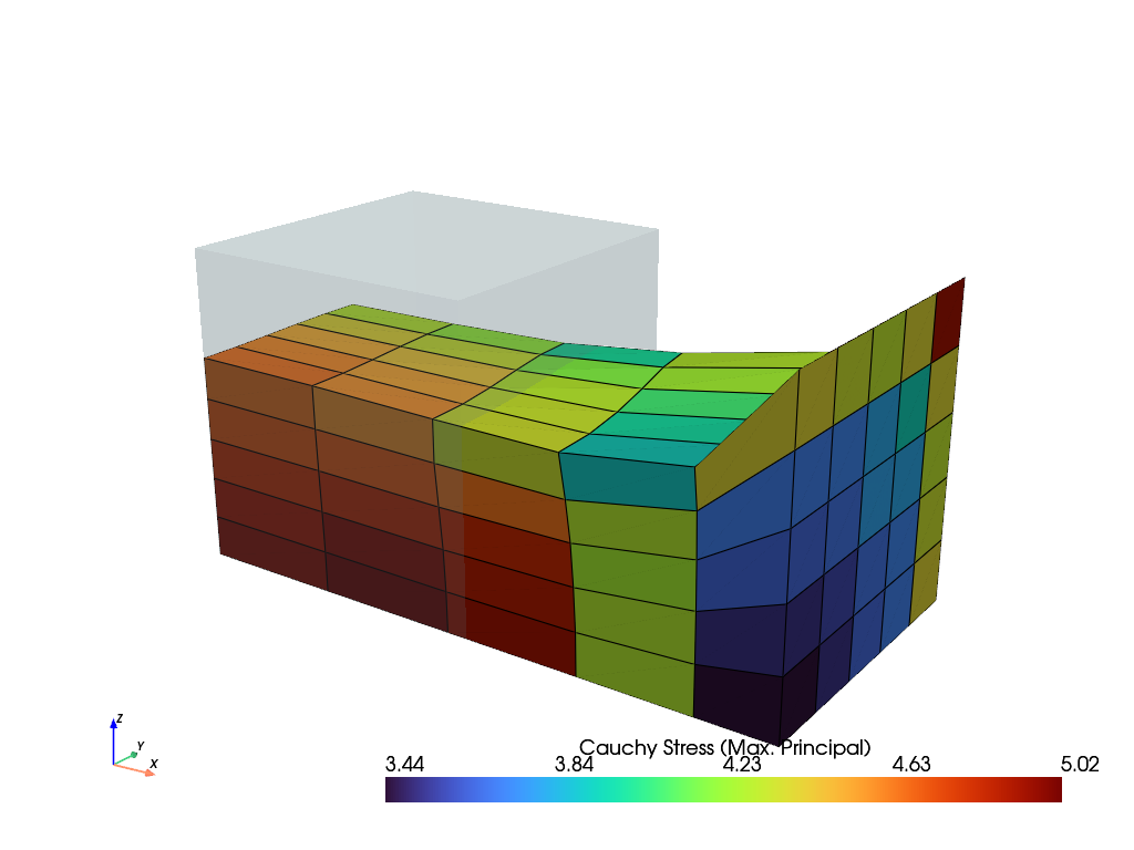
A view on the deformed mesh including the ContactRigidPlane is plotted.

>>> plotter = pv.Plotter()
>>>
>>> actor_1 = plotter.add_points(
...     mesh.points[contact.points] + displacement.values[contact.points],
...     point_size=16,
...     color="red",
... )
>>> actor_2 = plotter.add_points(
...     mesh.points[[contact.centerpoint]] + displacement.values[[contact.centerpoint]],
...     point_size=16,
...     color="green",
... )
>>> field.plot(
...     "Displacement",
...     component=None,
...     show_undeformed=False,
...     plotter=contact.plot(size=1.2, plotter=plotter),
...     clim=[0, 0.5],
... ).show()

contact_multipliers(contact)

plot(plotter=None, offset=0.0, show_edges=True, color='black', opacity=0.5, deformed=True, size=None, line_width=None, line_width_normal=None, show_point=True, show_line=True, sym=(False, False, False), **kwargs)

class felupe.mechanics.StateNearlyIncompressible(field)

A State with internal cell-wise constant dual fields for (nearly) incompressible solid bodies.

メモ

The internal fields \(p\) and \(\bar{J}\) are treated as internal fields, directly derived from the displacement field. Hence, these fields are not exported to the global degrees of freedom.

パラメータ:

field (FieldContainer) -- A field container with the displacement field.

参考

felupe.SolidBodyNearlyIncompressible

A (nearly) incompressible solid body with methods for the assembly of sparse vectors/matrices.

integrate_shape_function_gradient(parallel=False, out=None)

Integrated sub-block matrix containing the shape-functions gradient w.r.t. the deformed coordinates \(\boldsymbol{K}_{\boldsymbol{u}p}\).

\[\int_V \delta \boldsymbol{F} : \frac{\partial J}{\partial \boldsymbol{F}} ~ dV\ \Delta p \longrightarrow \boldsymbol{K}_{\boldsymbol{u}p}\]

volume()

Return the cell volumes of the deformed configuration.

\[v = \int_V J ~ dV\]

class felupe.mechanics.Assemble(vector=None, matrix=None, mass=None, multiplier=None)

A class with methods for assembling vectors and matrices of an Item.

class felupe.mechanics.Evaluate(gradient, hessian, stress=None, cauchy_stress=None, kirchhoff_stress=None)

A class with evaluate methods of an Item.

class felupe.mechanics.Results(stress=False, elasticity=False)

A class with intermediate results of an Item.

update_statevars()

class felupe.mechanics.UpdateItem(parent, key)

A helper class to update an item in the parent class when the value changes.

パラメータ:

• parent (object) -- The parent object that contains the item to be updated.

• key (str) -- The key of the item's parameter to be updated in the parent object.

update(value)