Models#
This page contains the core (hard-coded) constitutive material model formulations (not using automatic differentiation) for linear-elasticitiy, small-strain plasticity, hyperelasticity and pseudo-elasticity.
Poisson Equation
|
Laplace equation as hessian of one half of the second main invariant of the field gradient. |
Linear-Elasticity
|
Isotropic linear-elastic material formulation. |
Isotropic one-dimensional linear-elastic material formulation. |
|
|
Plane-stress isotropic linear-elastic material formulation. |
Plane-strain isotropic linear-elastic material formulation. |
|
Isotropic linear-elastic material formulation. |
|
|
Linear-elastic material formulation suitable for large-strain analyses based on the compressible Neo-Hookean material formulation. |
|
Orthotropic linear-elastic material formulation. |
Plasticity
Linear-elastic-plastic material formulation with linear isotropic hardening (return mapping algorithm). |
Hyperelasticity
|
Nearly-incompressible isotropic hyperelastic Neo-Hookean material formulation. |
|
Compressible isotropic hyperelastic Neo-Hookean material formulation. |
|
Ogden-Roxburgh Pseudo-Elastic material formulation for an isotropic treatment of the load-history dependent Mullins-softening of rubber-like materials. |
Mixed-Field Formulations \((\boldsymbol{u}, p, \bar{J})\)
|
Hu-Washizu hydrostatic-volumetric selective \((\boldsymbol{u},p,J)\) - three-field variation for nearly- incompressible material formulations. |
|
A nearly-incompressible material formulation to augment the distortional part of the strain energy function by a volumetric part and a constraint equation. |
Strain-based Materials
|
A strain-based user-defined material definition with a given function for the stress tensor and the (fourth-order) elasticity tensor. |
|
3D linear-elastic material formulation to be used in |
|
3D linear-elastic viscoelastic material formulation to be used in |
Linear-elastic-plastic material formulation with linear isotropic hardening (return mapping algorithm) to be used in |
Detailed API Reference
- class felupe.Laplace(multiplier=1.0)[ソース]#
Laplace equation as hessian of one half of the second main invariant of the field gradient.
- パラメータ:
multiplier (float, optional) -- A multiplier which scales the potential (default is 1.0).
メモ
The potential is given by the second main invariant of the field gradient w.r.t. the undeformed coordinates.
\[\psi = \frac{1}{2} \left( \boldsymbol{H} : \boldsymbol{H} \right)\]with the field gradient w.r.t. the undeformed coordinates.
\[\boldsymbol{H} = \frac{\partial \boldsymbol{u}}{\partial \boldsymbol{X}}\]サンプル
>>> import felupe as fem
>>>
>>> umat = fem.Laplace()
>>> ax = umat.plot()
- copy()#
Return a deep-copy of the constitutive material.
- function(x)[ソース]#
Evaluate the potential per unit undeformed volume.
- パラメータ:
x (list of ndarray) -- List with Deformation gradient \(\boldsymbol{F}\) as first item.
- 戻り値:
potential
- 戻り値の型:
ndarray of shape (...)
- gradient(x)[ソース]#
Evaluate the stress tensor.
- パラメータ:
x (list of ndarray) -- List with Deformation gradient \(\boldsymbol{F}\) as first item.
- 戻り値:
gradient of the potential w.r.t. the undeformed coordinates
- 戻り値の型:
ndarray of shape (n, m, ...)
- hessian(x)[ソース]#
Evaluate the elasticity tensor.
- パラメータ:
x (list of ndarray) -- List with Deformation gradient \(\boldsymbol{F}\) as first item.
- 戻り値:
hessian of the potential w.r.t. the undeformed coordinates
- 戻り値の型:
ndarray of shape (n, m, n, m, ...)
- is_stable(x, hessian=None)#
Return a boolean mask for stability of isotropic material model formulations.
At a given deformation gradient, a normal force is applied on each principal stretch direction. If the resulting incremental stretches are positive, the material model formulation is considered to be stable at the given deformation gradient.
- パラメータ:
x (list of ndarray) -- The list with input arguments. These contain the extracted fields of a
FieldContainer.hessian (ndarray or None, optional) -- Second partial derivative of the strain energy density function w.r.t. the deformation gradient. Default is None.
- 戻り値:
Boolean mask of stability.
- 戻り値の型:
ndarray
メモ
警告
This stability check will lead to a singular matrix for isotropic (hyperelastic) material model formulations without a volumetric part.
サンプル
First, let's check the stability of the Neo-Hookean material model formulation. The stability is evaluated on (valid) principal stretches of a biaxial deformation. All deformations are stable.
>>> import numpy as np
>>> import felupe as fem
>>>
>>> umat = fem.NeoHooke(mu=1.0, bulk=2.0)
>>> view = umat.view()
>>> λ = view.biaxial()[0]
>>>
>>> F = np.zeros((3, 3, 1, λ[0].size))
>>> for a in range(3):
...     F[a, a] = λ[a]
>>>
>>> umat.is_stable([F])
array([[ True,  True,  True,  True,  True,  True,  True,  True,  True,
         True,  True,  True,  True,  True,  True,  True]])
Now, let's check the stability of the Mooney-Rivlin material model formulation. The stability is evaluated on (valid) principal stretches of a biaxial deformation. Biaxial deformations are only stable up to a longitudinal stretch of 1.35.
>>> import numpy as np
>>> import felupe as fem
>>> import felupe.constitution.tensortrax as mat
>>>
>>> umat = fem.Hyperelastic(
...     mat.models.hyperelastic.mooney_rivlin,
...     C10=0.25,
...     C01=0.25,
... ) & fem.Volumetric(bulk=5000)
>>> view = umat.view()
>>> λ = view.biaxial()[0]
>>>
>>> F = np.zeros((3, 3, 1, λ[0].size))
>>> for a in range(3):
...     F[a, a] = λ[a]
>>>
>>> umat.is_stable([F])
array([[ True,  True,  True,  True,  True,  True,  True,  True, False,
        False, False, False, False, False, False, False]])
- optimize(ux=None, ps=None, bx=None, incompressible=False, relative=False, **kwargs)#
Optimize the material parameters by a least-squares fit on experimental stretch-stress data.
- パラメータ:
ux (array of shape (2, ...) or None, optional) -- Experimental uniaxial stretch and force-per-undeformed-area data (default is None).
ps (array of shape (2, ...) or None, optional) -- Experimental planar-shear stretch and force-per-undeformed-area data (default is None).
bx (array of shape (2, ...) or None, optional) -- Experimental biaxial stretch and force-per-undeformed-area data (default is None).
incompressible (bool, optional) -- A flag to enforce incompressible deformations (default is False).
relative (bool, optional) -- A flag to optimize relative instead of absolute residuals, i.e.
(predicted - observed) / observedinstead ofpredicted - observed(default is False).**kwargs (dict, optional) -- Optional keyword arguments are passed to
scipy.optimize.least_squares().
- 戻り値:
ConstitutiveMaterial -- A copy of the constitutive material with the optimized material parameters.
scipy.optimize.OptimizeResult -- Represents the optimization result.
メモ
警告
At least one load case, i.e. one of the arguments
ux,psorbxmust not beNone.注釈
For JAX-based materials, double-precision is required to optimize material parameters.
import jax

jax.config.update("jax_enable_x64", True)
The vector of residuals is given in Eq. (3) in case of absolute residuals
(1)#\[ \begin{align}\begin{aligned}\begin{split}\boldsymbol{r} &= \begin{bmatrix} \boldsymbol{r}_\text{ux} \\ \boldsymbol{r}_\text{ps} \\ \boldsymbol{r}_\text{bx} \end{bmatrix}\end{split}\\r_\text{ux}(\lambda_i) &= P_\text{ux}(\lambda_i) - P_\text{ux, observed}(\lambda_i)\\r_\text{ps}(\lambda_i) &= P_\text{ps}(\lambda_i) - P_\text{ps, observed}(\lambda_i)\\r_\text{bx}(\lambda_i) &= P_\text{bx}(\lambda_i) - P_\text{bx, observed}(\lambda_i)\end{aligned}\end{align} \]and in Eq. (4) in case of relative residuals.
(2)#\[ \begin{align}\begin{aligned}\begin{split}\boldsymbol{r} &= \begin{bmatrix} \boldsymbol{r}_\text{ux} \\ \boldsymbol{r}_\text{ps} \\ \boldsymbol{r}_\text{bx} \end{bmatrix}\end{split}\\r_\text{ux}(\lambda_i) &= \frac{ P_\text{ux}(\lambda_i) - P_\text{ux, observed}(\lambda_i)}{ P_\text{ux, observed}(\lambda_i) }\\r_\text{ps}(\lambda_i) &= \frac{ P_\text{ps}(\lambda_i) - P_\text{ps, observed}(\lambda_i)}{ P_\text{ps, observed}(\lambda_i) }\\r_\text{bx}(\lambda_i) &= \frac{ P_\text{bx}(\lambda_i) - P_\text{bx, observed}(\lambda_i)}{ P_\text{bx, observed}(\lambda_i) }\end{aligned}\end{align} \]サンプル
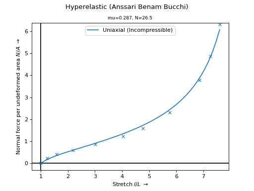
The
Anssari-Benam Bucchimaterial model formulation is best-fitted on Treloar's uniaxial and biaxial tension data [1]_.>>> import numpy as np >>> import felupe as fem >>> >>> λ, P = np.array( ... [ ... [1.000, 0.00], ... [1.240, 2.30], ... [1.585, 4.16], ... [2.180, 6.00], ... [3.020, 8.80], ... [4.030, 12.5], ... [4.760, 16.2], ... [5.750, 23.6], ... [6.850, 38.5], ... [7.250, 49.6], ... [7.600, 64.4], ... ] ... ).T * np.array([[1.0], [0.0980665]]) >>> >>> umat = fem.Hyperelastic(fem.anssari_benam_bucchi) >>> umat_new, res = umat.optimize( ... ux=[λ, P], incompressible=True, relative=True ... ) >>> >>> ux = np.linspace(λ.min(), λ.max(), num=50) >>> ax = umat_new.plot(incompressible=True, ux=ux, bx=None, ps=None) >>> ax.plot(λ, P, "C0x")

参考
scipy.optimize.least_squaresSolve a nonlinear least-squares problem with bounds on the variables.
参照
- plot(incompressible=False, **kwargs)#
Return a plot with normal force per undeformed area vs. stretch curves for the elementary homogeneous deformations uniaxial tension/compression, planar shear and biaxial tension of a given isotropic material formulation.
- パラメータ:
incompressible (bool, optional) -- A flag to enforce views on incompressible deformations (default is False).
**kwargs (dict, optional) -- Optional keyword-arguments for
ViewMaterialorViewMaterialIncompressible.
- 戻り値の型:
参考
felupe.ViewMaterialCreate views on normal force per undeformed area vs. stretch curves for the elementary homogeneous deformations uniaxial tension/compression, planar shear and biaxial tension of a given isotropic material formulation.
felupe.ViewMaterialIncompressibleCreate views on normal force per undeformed area vs. stretch curves for the elementary homogeneous incompressible deformations uniaxial tension/compression, planar shear and biaxial tension of a given isotropic material formulation.
- screenshot(filename='umat.png', incompressible=False, **kwargs)#
Save a screenshot with normal force per undeformed area vs. stretch curves for the elementary homogeneous deformations uniaxial tension/compression, planar shear and biaxial tension of a given isotropic material formulation.
- パラメータ:
filename (str, optional) -- The filename of the screenshot (default is "umat.png").
incompressible (bool, optional) -- A flag to enforce views on incompressible deformations (default is False).
**kwargs (dict, optional) -- Optional keyword-arguments for
ViewMaterialorViewMaterialIncompressible.
- 戻り値の型:
参考
felupe.ViewMaterialCreate views on normal force per undeformed area vs. stretch curves for the elementary homogeneous deformations uniaxial tension/compression, planar shear and biaxial tension of a given isotropic material formulation.
felupe.ViewMaterialIncompressibleCreate views on normal force per undeformed area vs. stretch curves for the elementary homogeneous incompressible deformations uniaxial tension/compression, planar shear and biaxial tension of a given isotropic material formulation.
- view(incompressible=False, **kwargs)#
Create views on normal force per undeformed area vs. stretch curves for the elementary homogeneous deformations uniaxial tension/compression, planar shear and biaxial tension of a given isotropic material formulation.
- パラメータ:
incompressible (bool, optional) -- A flag to enforce views on incompressible deformations (default is False).
**kwargs (dict, optional) -- Optional keyword-arguments for
ViewMaterialorViewMaterialIncompressible.
- 戻り値の型:
参考
felupe.ViewMaterialCreate views on normal force per undeformed area vs. stretch curves for the elementary homogeneous deformations uniaxial tension/compression, planar shear and biaxial tension of a given isotropic material formulation.
felupe.ViewMaterialIncompressibleCreate views on normal force per undeformed area vs. stretch curves for the elementary homogeneous incompressible deformations uniaxial tension/compression, planar shear and biaxial tension of a given isotropic material formulation.
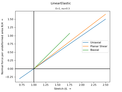
- class felupe.LinearElastic(E, nu)[ソース]#
Isotropic linear-elastic material formulation.
メモ
The stress-strain relation of the linear-elastic material formulation is given in Eq. (3)
(3)#\[\begin{split}\begin{bmatrix} \sigma_{11} \\ \sigma_{22} \\ \sigma_{33} \\ \sigma_{12} \\ \sigma_{23} \\ \sigma_{31} \end{bmatrix} = \frac{E}{(1+\nu)(1-2\nu)}\begin{bmatrix} 1-\nu & \nu & \nu & 0 & 0 & 0\\ \nu & 1-\nu & \nu & 0 & 0 & 0\\ \nu & \nu & 1-\nu & 0 & 0 & 0\\ 0 & 0 & 0 & \frac{1-2\nu}{2} & 0 & 0 \\ 0 & 0 & 0 & 0 & \frac{1-2\nu}{2} & 0 \\ 0 & 0 & 0 & 0 & 0 & \frac{1-2\nu}{2} \end{bmatrix} \cdot \begin{bmatrix} \varepsilon_{11} \\ \varepsilon_{22} \\ \varepsilon_{33} \\ 2 \varepsilon_{12} \\ 2 \varepsilon_{23} \\ 2 \varepsilon_{31} \end{bmatrix}\end{split}\]with the small-strain tensor from Eq. (4).
(4)#\[\boldsymbol{\varepsilon} = \frac{1}{2} \left( \frac{\partial \boldsymbol{u}} {\partial \boldsymbol{X}} + \left( \frac{\partial \boldsymbol{u}} {\partial \boldsymbol{X}} \right)^T \right)\]警告
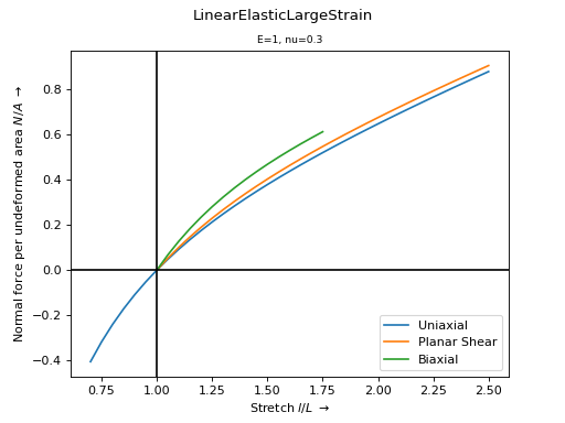
This material formulation must not be used in analyses where large rotations, large displacements or large strains occur. In this case, consider using a
Hyperelasticmaterial formulation instead.LinearElasticLargeStrainis based on a compressible version of the Neo-Hookean material formulation and is safe to use for large rotations, large displacements and large strains.サンプル
>>> import felupe as fem
>>>
>>> umat = fem.LinearElastic(E=1, nu=0.3)
>>> ax = umat.plot()
参考
felupe.LinearElasticLargeStrainLinear-elastic material formulation suitable for large-strain analyses based on the compressible Neo-Hookean material formulation.
felupe.HyperelasticA hyperelastic material definition with a given function for the strain energy density function per unit undeformed volume with automatic differentiation.
- copy()#
Return a deep-copy of the constitutive material.
- gradient(x)[ソース]#
Evaluate the stress tensor (as a function of the deformation gradient).
- パラメータ:
x (list of ndarray) -- List with Deformation gradient \(\boldsymbol{F}\) (3x3) as first item.
- 戻り値:
Stress tensor (3x3)
- 戻り値の型:
ndarray
- hessian(x=None, shape=(1, 1), dtype=None)[ソース]#
Evaluate the elasticity tensor. The Deformation gradient is only used for the shape of the trailing axes.
- is_stable(x, hessian=None)#
Return a boolean mask for stability of isotropic material model formulations.
At a given deformation gradient, a normal force is applied on each principal stretch direction. If the resulting incremental stretches are positive, the material model formulation is considered to be stable at the given deformation gradient.
- パラメータ:
x (list of ndarray) -- The list with input arguments. These contain the extracted fields of a
FieldContainer.hessian (ndarray or None, optional) -- Second partial derivative of the strain energy density function w.r.t. the deformation gradient. Default is None.
- 戻り値:
Boolean mask of stability.
- 戻り値の型:
ndarray
メモ
警告
This stability check will lead to a singular matrix for isotropic (hyperelastic) material model formulations without a volumetric part.
サンプル
First, let's check the stability of the Neo-Hookean material model formulation. The stability is evaluated on (valid) principal stretches of a biaxial deformation. All deformations are stable.
>>> import numpy as np
>>> import felupe as fem
>>>
>>> umat = fem.NeoHooke(mu=1.0, bulk=2.0)
>>> view = umat.view()
>>> λ = view.biaxial()[0]
>>>
>>> F = np.zeros((3, 3, 1, λ[0].size))
>>> for a in range(3):
...     F[a, a] = λ[a]
>>>
>>> umat.is_stable([F])
array([[ True,  True,  True,  True,  True,  True,  True,  True,  True,
         True,  True,  True,  True,  True,  True,  True]])
Now, let's check the stability of the Mooney-Rivlin material model formulation. The stability is evaluated on (valid) principal stretches of a biaxial deformation. Biaxial deformations are only stable up to a longitudinal stretch of 1.35.
>>> import numpy as np
>>> import felupe as fem
>>> import felupe.constitution.tensortrax as mat
>>>
>>> umat = fem.Hyperelastic(
...     mat.models.hyperelastic.mooney_rivlin,
...     C10=0.25,
...     C01=0.25,
... ) & fem.Volumetric(bulk=5000)
>>> view = umat.view()
>>> λ = view.biaxial()[0]
>>>
>>> F = np.zeros((3, 3, 1, λ[0].size))
>>> for a in range(3):
...     F[a, a] = λ[a]
>>>
>>> umat.is_stable([F])
array([[ True,  True,  True,  True,  True,  True,  True,  True, False,
        False, False, False, False, False, False, False]])
- optimize(ux=None, ps=None, bx=None, incompressible=False, relative=False, **kwargs)#
Optimize the material parameters by a least-squares fit on experimental stretch-stress data.
- パラメータ:
ux (array of shape (2, ...) or None, optional) -- Experimental uniaxial stretch and force-per-undeformed-area data (default is None).
ps (array of shape (2, ...) or None, optional) -- Experimental planar-shear stretch and force-per-undeformed-area data (default is None).
bx (array of shape (2, ...) or None, optional) -- Experimental biaxial stretch and force-per-undeformed-area data (default is None).
incompressible (bool, optional) -- A flag to enforce incompressible deformations (default is False).
relative (bool, optional) -- A flag to optimize relative instead of absolute residuals, i.e.
(predicted - observed) / observedinstead ofpredicted - observed(default is False).**kwargs (dict, optional) -- Optional keyword arguments are passed to
scipy.optimize.least_squares().
- 戻り値:
ConstitutiveMaterial -- A copy of the constitutive material with the optimized material parameters.
scipy.optimize.OptimizeResult -- Represents the optimization result.
メモ
警告
At least one load case, i.e. one of the arguments
ux,psorbxmust not beNone.注釈
For JAX-based materials, double-precision is required to optimize material parameters.
import jax

jax.config.update("jax_enable_x64", True)
The vector of residuals is given in Eq. (3) in case of absolute residuals
(5)#\[ \begin{align}\begin{aligned}\begin{split}\boldsymbol{r} &= \begin{bmatrix} \boldsymbol{r}_\text{ux} \\ \boldsymbol{r}_\text{ps} \\ \boldsymbol{r}_\text{bx} \end{bmatrix}\end{split}\\r_\text{ux}(\lambda_i) &= P_\text{ux}(\lambda_i) - P_\text{ux, observed}(\lambda_i)\\r_\text{ps}(\lambda_i) &= P_\text{ps}(\lambda_i) - P_\text{ps, observed}(\lambda_i)\\r_\text{bx}(\lambda_i) &= P_\text{bx}(\lambda_i) - P_\text{bx, observed}(\lambda_i)\end{aligned}\end{align} \]and in Eq. (4) in case of relative residuals.
(6)#\[ \begin{align}\begin{aligned}\begin{split}\boldsymbol{r} &= \begin{bmatrix} \boldsymbol{r}_\text{ux} \\ \boldsymbol{r}_\text{ps} \\ \boldsymbol{r}_\text{bx} \end{bmatrix}\end{split}\\r_\text{ux}(\lambda_i) &= \frac{ P_\text{ux}(\lambda_i) - P_\text{ux, observed}(\lambda_i)}{ P_\text{ux, observed}(\lambda_i) }\\r_\text{ps}(\lambda_i) &= \frac{ P_\text{ps}(\lambda_i) - P_\text{ps, observed}(\lambda_i)}{ P_\text{ps, observed}(\lambda_i) }\\r_\text{bx}(\lambda_i) &= \frac{ P_\text{bx}(\lambda_i) - P_\text{bx, observed}(\lambda_i)}{ P_\text{bx, observed}(\lambda_i) }\end{aligned}\end{align} \]サンプル
The
Anssari-Benam Bucchimaterial model formulation is best-fitted on Treloar's uniaxial and biaxial tension data [1]_.>>> import numpy as np >>> import felupe as fem >>> >>> λ, P = np.array( ... [ ... [1.000, 0.00], ... [1.240, 2.30], ... [1.585, 4.16], ... [2.180, 6.00], ... [3.020, 8.80], ... [4.030, 12.5], ... [4.760, 16.2], ... [5.750, 23.6], ... [6.850, 38.5], ... [7.250, 49.6], ... [7.600, 64.4], ... ] ... ).T * np.array([[1.0], [0.0980665]]) >>> >>> umat = fem.Hyperelastic(fem.anssari_benam_bucchi) >>> umat_new, res = umat.optimize( ... ux=[λ, P], incompressible=True, relative=True ... ) >>> >>> ux = np.linspace(λ.min(), λ.max(), num=50) >>> ax = umat_new.plot(incompressible=True, ux=ux, bx=None, ps=None) >>> ax.plot(λ, P, "C0x")
参考
scipy.optimize.least_squaresSolve a nonlinear least-squares problem with bounds on the variables.
参照
- plot(incompressible=False, **kwargs)#
Return a plot with normal force per undeformed area vs. stretch curves for the elementary homogeneous deformations uniaxial tension/compression, planar shear and biaxial tension of a given isotropic material formulation.
- パラメータ:
incompressible (bool, optional) -- A flag to enforce views on incompressible deformations (default is False).
**kwargs (dict, optional) -- Optional keyword-arguments for
ViewMaterialorViewMaterialIncompressible.
- 戻り値の型:
参考
felupe.ViewMaterialCreate views on normal force per undeformed area vs. stretch curves for the elementary homogeneous deformations uniaxial tension/compression, planar shear and biaxial tension of a given isotropic material formulation.
felupe.ViewMaterialIncompressibleCreate views on normal force per undeformed area vs. stretch curves for the elementary homogeneous incompressible deformations uniaxial tension/compression, planar shear and biaxial tension of a given isotropic material formulation.
- screenshot(filename='umat.png', incompressible=False, **kwargs)#
Save a screenshot with normal force per undeformed area vs. stretch curves for the elementary homogeneous deformations uniaxial tension/compression, planar shear and biaxial tension of a given isotropic material formulation.
- パラメータ:
filename (str, optional) -- The filename of the screenshot (default is "umat.png").
incompressible (bool, optional) -- A flag to enforce views on incompressible deformations (default is False).
**kwargs (dict, optional) -- Optional keyword-arguments for
ViewMaterialorViewMaterialIncompressible.
- 戻り値の型:
参考
felupe.ViewMaterialCreate views on normal force per undeformed area vs. stretch curves for the elementary homogeneous deformations uniaxial tension/compression, planar shear and biaxial tension of a given isotropic material formulation.
felupe.ViewMaterialIncompressibleCreate views on normal force per undeformed area vs. stretch curves for the elementary homogeneous incompressible deformations uniaxial tension/compression, planar shear and biaxial tension of a given isotropic material formulation.
- view(incompressible=False, **kwargs)#
Create views on normal force per undeformed area vs. stretch curves for the elementary homogeneous deformations uniaxial tension/compression, planar shear and biaxial tension of a given isotropic material formulation.
- パラメータ:
incompressible (bool, optional) -- A flag to enforce views on incompressible deformations (default is False).
**kwargs (dict, optional) -- Optional keyword-arguments for
ViewMaterialorViewMaterialIncompressible.
- 戻り値の型:
参考
felupe.ViewMaterialCreate views on normal force per undeformed area vs. stretch curves for the elementary homogeneous deformations uniaxial tension/compression, planar shear and biaxial tension of a given isotropic material formulation.
felupe.ViewMaterialIncompressibleCreate views on normal force per undeformed area vs. stretch curves for the elementary homogeneous incompressible deformations uniaxial tension/compression, planar shear and biaxial tension of a given isotropic material formulation.
- class felupe.LinearElastic1D(E)[ソース]#
Isotropic one-dimensional linear-elastic material formulation.
- パラメータ:
E (float) -- Young's modulus.
メモ
The stress-stretch relation of the linear-elastic material formulation is given in Eq. (7)
(7)#\[\sigma = E\ \left(\lambda - 1 \right)\]with the stretch from Eq. (8).
(8)#\[\lambda = \frac{l}{L}\]サンプル
>>> import felupe as fem
>>>
>>> umat = fem.LinearElastic1D(E=1)
>>> ax = umat.plot()
- copy()#
Return a deep-copy of the constitutive material.
- gradient(x, out=None)[ソース]#
Evaluate the stress (as a function of the stretch).
- パラメータ:
x (list of ndarray) -- List with the stretch \(\lambda\) as first item.
out (ndarray or None, optional) -- A location into which the result is stored (default is None). Not implemented.
- 戻り値:
Stress
- 戻り値の型:
ndarray
- hessian(x=None, shape=(1,), dtype=None, out=None)[ソース]#
Evaluate the elasticity. The stretch is only used for the shape of the trailing axes.
- パラメータ:
x (list of ndarray, optional) -- List with stretch \(\lambda\) as first item (default is None).
shape (tuple of int, optional) -- Tuple with shape of the trailing axes (default is (1,)).
out (ndarray or None, optional) -- A location into which the result is stored (default is None). Not implemented.
- 戻り値:
Elasticity
- 戻り値の型:
ndarray
- is_stable(x, hessian=None)#
Return a boolean mask for stability of isotropic material model formulations.
At a given deformation gradient, a normal force is applied on each principal stretch direction. If the resulting incremental stretches are positive, the material model formulation is considered to be stable at the given deformation gradient.
- パラメータ:
x (list of ndarray) -- The list with input arguments. These contain the extracted fields of a
FieldContainer.hessian (ndarray or None, optional) -- Second partial derivative of the strain energy density function w.r.t. the deformation gradient. Default is None.
- 戻り値:
Boolean mask of stability.
- 戻り値の型:
ndarray
メモ
警告
This stability check will lead to a singular matrix for isotropic (hyperelastic) material model formulations without a volumetric part.
サンプル
First, let's check the stability of the Neo-Hookean material model formulation. The stability is evaluated on (valid) principal stretches of a biaxial deformation. All deformations are stable.
>>> import numpy as np
>>> import felupe as fem
>>>
>>> umat = fem.NeoHooke(mu=1.0, bulk=2.0)
>>> view = umat.view()
>>> λ = view.biaxial()[0]
>>>
>>> F = np.zeros((3, 3, 1, λ[0].size))
>>> for a in range(3):
...     F[a, a] = λ[a]
>>>
>>> umat.is_stable([F])
array([[ True,  True,  True,  True,  True,  True,  True,  True,  True,
         True,  True,  True,  True,  True,  True,  True]])
Now, let's check the stability of the Mooney-Rivlin material model formulation. The stability is evaluated on (valid) principal stretches of a biaxial deformation. Biaxial deformations are only stable up to a longitudinal stretch of 1.35.
>>> import numpy as np
>>> import felupe as fem
>>> import felupe.constitution.tensortrax as mat
>>>
>>> umat = fem.Hyperelastic(
...     mat.models.hyperelastic.mooney_rivlin,
...     C10=0.25,
...     C01=0.25,
... ) & fem.Volumetric(bulk=5000)
>>> view = umat.view()
>>> λ = view.biaxial()[0]
>>>
>>> F = np.zeros((3, 3, 1, λ[0].size))
>>> for a in range(3):
...     F[a, a] = λ[a]
>>>
>>> umat.is_stable([F])
array([[ True,  True,  True,  True,  True,  True,  True,  True, False,
        False, False, False, False, False, False, False]])
- optimize(ux=None, ps=None, bx=None, incompressible=False, relative=False, **kwargs)#
Optimize the material parameters by a least-squares fit on experimental stretch-stress data.
- パラメータ:
ux (array of shape (2, ...) or None, optional) -- Experimental uniaxial stretch and force-per-undeformed-area data (default is None).
ps (array of shape (2, ...) or None, optional) -- Experimental planar-shear stretch and force-per-undeformed-area data (default is None).
bx (array of shape (2, ...) or None, optional) -- Experimental biaxial stretch and force-per-undeformed-area data (default is None).
incompressible (bool, optional) -- A flag to enforce incompressible deformations (default is False).
relative (bool, optional) -- A flag to optimize relative instead of absolute residuals, i.e.
(predicted - observed) / observedinstead ofpredicted - observed(default is False).**kwargs (dict, optional) -- Optional keyword arguments are passed to
scipy.optimize.least_squares().
- 戻り値:
ConstitutiveMaterial -- A copy of the constitutive material with the optimized material parameters.
scipy.optimize.OptimizeResult -- Represents the optimization result.
メモ
警告
At least one load case, i.e. one of the arguments
ux,psorbxmust not beNone.注釈
For JAX-based materials, double-precision is required to optimize material parameters.
import jax

jax.config.update("jax_enable_x64", True)
The vector of residuals is given in Eq. (3) in case of absolute residuals
(9)#\[ \begin{align}\begin{aligned}\begin{split}\boldsymbol{r} &= \begin{bmatrix} \boldsymbol{r}_\text{ux} \\ \boldsymbol{r}_\text{ps} \\ \boldsymbol{r}_\text{bx} \end{bmatrix}\end{split}\\r_\text{ux}(\lambda_i) &= P_\text{ux}(\lambda_i) - P_\text{ux, observed}(\lambda_i)\\r_\text{ps}(\lambda_i) &= P_\text{ps}(\lambda_i) - P_\text{ps, observed}(\lambda_i)\\r_\text{bx}(\lambda_i) &= P_\text{bx}(\lambda_i) - P_\text{bx, observed}(\lambda_i)\end{aligned}\end{align} \]and in Eq. (4) in case of relative residuals.
(10)#\[ \begin{align}\begin{aligned}\begin{split}\boldsymbol{r} &= \begin{bmatrix} \boldsymbol{r}_\text{ux} \\ \boldsymbol{r}_\text{ps} \\ \boldsymbol{r}_\text{bx} \end{bmatrix}\end{split}\\r_\text{ux}(\lambda_i) &= \frac{ P_\text{ux}(\lambda_i) - P_\text{ux, observed}(\lambda_i)}{ P_\text{ux, observed}(\lambda_i) }\\r_\text{ps}(\lambda_i) &= \frac{ P_\text{ps}(\lambda_i) - P_\text{ps, observed}(\lambda_i)}{ P_\text{ps, observed}(\lambda_i) }\\r_\text{bx}(\lambda_i) &= \frac{ P_\text{bx}(\lambda_i) - P_\text{bx, observed}(\lambda_i)}{ P_\text{bx, observed}(\lambda_i) }\end{aligned}\end{align} \]サンプル
The
Anssari-Benam Bucchimaterial model formulation is best-fitted on Treloar's uniaxial and biaxial tension data [1]_.>>> import numpy as np >>> import felupe as fem >>> >>> λ, P = np.array( ... [ ... [1.000, 0.00], ... [1.240, 2.30], ... [1.585, 4.16], ... [2.180, 6.00], ... [3.020, 8.80], ... [4.030, 12.5], ... [4.760, 16.2], ... [5.750, 23.6], ... [6.850, 38.5], ... [7.250, 49.6], ... [7.600, 64.4], ... ] ... ).T * np.array([[1.0], [0.0980665]]) >>> >>> umat = fem.Hyperelastic(fem.anssari_benam_bucchi) >>> umat_new, res = umat.optimize( ... ux=[λ, P], incompressible=True, relative=True ... ) >>> >>> ux = np.linspace(λ.min(), λ.max(), num=50) >>> ax = umat_new.plot(incompressible=True, ux=ux, bx=None, ps=None) >>> ax.plot(λ, P, "C0x")

参考
scipy.optimize.least_squaresSolve a nonlinear least-squares problem with bounds on the variables.
参照
- plot(incompressible=False, **kwargs)#
Return a plot with normal force per undeformed area vs. stretch curves for the elementary homogeneous deformations uniaxial tension/compression, planar shear and biaxial tension of a given isotropic material formulation.
- パラメータ:
incompressible (bool, optional) -- A flag to enforce views on incompressible deformations (default is False).
**kwargs (dict, optional) -- Optional keyword-arguments for
ViewMaterialorViewMaterialIncompressible.
- 戻り値の型:
参考
felupe.ViewMaterialCreate views on normal force per undeformed area vs. stretch curves for the elementary homogeneous deformations uniaxial tension/compression, planar shear and biaxial tension of a given isotropic material formulation.
felupe.ViewMaterialIncompressibleCreate views on normal force per undeformed area vs. stretch curves for the elementary homogeneous incompressible deformations uniaxial tension/compression, planar shear and biaxial tension of a given isotropic material formulation.
- screenshot(filename='umat.png', incompressible=False, **kwargs)#
Save a screenshot with normal force per undeformed area vs. stretch curves for the elementary homogeneous deformations uniaxial tension/compression, planar shear and biaxial tension of a given isotropic material formulation.
- パラメータ:
filename (str, optional) -- The filename of the screenshot (default is "umat.png").
incompressible (bool, optional) -- A flag to enforce views on incompressible deformations (default is False).
**kwargs (dict, optional) -- Optional keyword-arguments for
ViewMaterialorViewMaterialIncompressible.
- 戻り値の型:
参考
felupe.ViewMaterialCreate views on normal force per undeformed area vs. stretch curves for the elementary homogeneous deformations uniaxial tension/compression, planar shear and biaxial tension of a given isotropic material formulation.
felupe.ViewMaterialIncompressibleCreate views on normal force per undeformed area vs. stretch curves for the elementary homogeneous incompressible deformations uniaxial tension/compression, planar shear and biaxial tension of a given isotropic material formulation.
- view(incompressible=False, **kwargs)#
Create views on normal force per undeformed area vs. stretch curves for the elementary homogeneous deformations uniaxial tension/compression, planar shear and biaxial tension of a given isotropic material formulation.
- パラメータ:
incompressible (bool, optional) -- A flag to enforce views on incompressible deformations (default is False).
**kwargs (dict, optional) -- Optional keyword-arguments for
ViewMaterialorViewMaterialIncompressible.
- 戻り値の型:
参考
felupe.ViewMaterialCreate views on normal force per undeformed area vs. stretch curves for the elementary homogeneous deformations uniaxial tension/compression, planar shear and biaxial tension of a given isotropic material formulation.
felupe.ViewMaterialIncompressibleCreate views on normal force per undeformed area vs. stretch curves for the elementary homogeneous incompressible deformations uniaxial tension/compression, planar shear and biaxial tension of a given isotropic material formulation.
- felupe.linear_elastic(dε, εn, σn, ζn, λ, μ, **kwargs)[ソース]#
3D linear-elastic material formulation to be used in
MaterialStrain.- パラメータ:
dε (ndarray) -- Strain increment.
εn (ndarray) -- Old strain tensor.
σn (ndarray) -- Old stress tensor.
ζn (list) -- List of old state variables.
λ (float) -- First Lamé-constant.
μ (float) -- Second Lamé-constant (shear modulus).
**kwargs --
Additional keyword arguments.
- tangentbool
A flag to evaluate the elasticity tensor.
- 戻り値:
dσdε (ndarray) -- Elasticity tensor.
σ (ndarray) -- (New) stress tensor.
ζ (list) -- List of new state variables.
メモ
Given state in point \(\boldsymbol{x} (\boldsymbol{\sigma}_n)\) (valid).
Given strain increment \(\Delta\boldsymbol{\varepsilon}\), so that \(\boldsymbol{\varepsilon} = \boldsymbol{\varepsilon}_n + \Delta\boldsymbol{\varepsilon}\).
Evaluation of the stress \(\boldsymbol{\sigma}\) and the algorithmic consistent tangent modulus \(\mathbb{C}\) (=``dσdε``).
\[ \begin{align}\begin{aligned}\mathbb{C} &= \lambda \ \boldsymbol{1} \otimes \boldsymbol{1} + 2 \mu \ \boldsymbol{1} \odot \boldsymbol{1}\\\boldsymbol{\sigma} &= \boldsymbol{\sigma}_n + \mathbb{C} : \Delta\boldsymbol{\varepsilon}\end{aligned}\end{align} \]
サンプル
>>> import felupe as fem
>>>
>>> umat = fem.MaterialStrain(material=fem.linear_elastic, λ=2.0, μ=1.0)
>>> ax = umat.plot()

参考
MaterialStrainA strain-based user-defined material definition with a given function for the stress tensor and the (fourth-order) elasticity tensor.
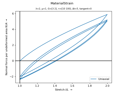
- felupe.linear_elastic_viscoelastic(dε, εn, σn, ζn, λ, μ, G, τ, Δt, **kwargs)[ソース]#
3D linear-elastic viscoelastic material formulation to be used in
MaterialStrain.- パラメータ:
dε (ndarray) -- Strain increment.
εn (ndarray) -- Old strain tensor.
σn (ndarray) -- Old stress tensor.
ζn (list) -- List of old state variables.
λ (float) -- First Lamé-constant.
μ (float) -- Second Lamé-constant (shear modulus).
G (list of float) -- List of deviatoric viscoelastic shear moduli.
τ (list of float) -- List of time constants for deviatoric viscoelastic shear moduli.
Δt (float) -- Time increment.
**kwargs --
Additional keyword arguments.
- tangentbool
A flag to evaluate the elasticity tensor.
- 戻り値:
dσdε (ndarray) -- Elasticity tensor.
σ (ndarray) -- (New) stress tensor.
ζ (list) -- List of new state variables.
メモ
The stress consists of a long-term elastic and a deviatoric viscoelastic stress part, see Eq. (11).
(11)#\[\boldsymbol{\sigma} = \boldsymbol{\sigma}_e + \boldsymbol{\sigma}_v\]The long-term elastic part is given in Eq. (12).
(12)#\[\boldsymbol{\sigma}_e = 2 \mu\ \boldsymbol{\varepsilon} + \lambda \operatorname{tr}(\boldsymbol{\varepsilon}) \boldsymbol{1}\]The i-th viscous part is given in Eq. (13),
(13)#\[ \begin{align}\begin{aligned}\dot{\boldsymbol{\sigma}}_{v,i} + \frac{1}{\tau_i} \boldsymbol{\sigma}_{v,i} &= 2 G_i \operatorname{dev}\left( \dot{\boldsymbol{\varepsilon}} \right)\\\boldsymbol{\sigma}_{v,i} &= a_i\ \boldsymbol{\sigma}_{v,i}^n + b_i \operatorname{dev} \left( \boldsymbol{\varepsilon} - \boldsymbol{\varepsilon}_n \right)\end{aligned}\end{align} \]with the coefficients as denoted in Eq. (14).
(14)#\[ \begin{align}\begin{aligned}a_i &= \exp \left( -\Delta t / \tau_i \right)\\b_i &= \frac{2 G_i\ \tau_i (1 - a_i)}{\Delta t}\end{aligned}\end{align} \]The total fourth-order elasticity tensor is given in Eq. (15).
(15)#\[\mathbb{C} = 2 \bar{\mu} \ \boldsymbol{1} \odot \boldsymbol{1} + \bar{\lambda}\ \boldsymbol{1} \otimes \boldsymbol{1}\]The effective coefficients are summarized in Eq. (16).
(16)#\[ \begin{align}\begin{aligned}\bar{\mu} &= \mu + \sum_{i=1}^N \frac{b_i}{2}\\\bar{\lambda} &= \lambda - \frac{2}{3} \left( \bar{\mu} - \mu \right)\end{aligned}\end{align} \]サンプル
>>> import felupe as fem
>>>
>>> umat = fem.MaterialStrain(
...     material=fem.linear_elastic_viscoelastic,
...     λ=2.0,
...     μ=1.0,
...     G=[3.0, 2.0],
...     τ=[10.0, 100.0],
...     Δt=5.0,
...     statevars=((2, 3, 3),),
... )
>>> ux = fem.math.linsteps([1, 2, 1, 2, 1, 2, 1], num=20)
>>> ax = umat.plot(ux=ux, bx=None, ps=None)
参考
MaterialStrainA strain-based user-defined material definition with a given function for the stress tensor and the (fourth-order) elasticity tensor.
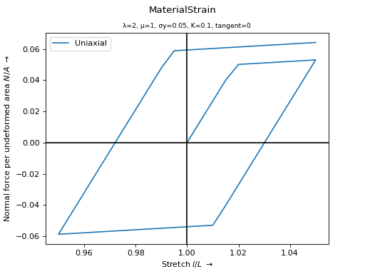
- felupe.linear_elastic_plastic_isotropic_hardening(dε, εn, σn, ζn, λ, μ, σy, K, **kwargs)[ソース]#
Linear-elastic-plastic material formulation with linear isotropic hardening (return mapping algorithm) to be used in
MaterialStrain.- パラメータ:
dε (ndarray) -- Strain increment.
εn (ndarray) -- Old strain tensor.
σn (ndarray) -- Old stress tensor.
ζn (list) -- List of old state variables.
λ (float) -- First Lamé-constant.
μ (float) -- Second Lamé-constant (shear modulus).
σy (float) -- Initial yield stress.
K (float) -- Isotropic hardening modulus.
**kwargs --
Additional keyword arguments.
- tangentbool
A flag to evaluate the elasticity tensor.
- 戻り値:
dσdε (ndarray) -- Algorithmic consistent elasticity tensor.
σ (ndarray) -- (New) stress tensor.
ζ (list) -- List of new state variables.
メモ
Given state in point \(x (\sigma_n, \zeta_n=[\varepsilon^p_n, \alpha_n])\) (valid).
Given strain increment \(\Delta\varepsilon\), so that \(\varepsilon = \varepsilon_n + \Delta\varepsilon\).
Evaluation of the hypothetic trial state:
\[ \begin{align}\begin{aligned}\mathbb{C} &= \lambda\ \boldsymbol{1} \otimes \boldsymbol{1} + 2 \mu\ \boldsymbol{1} \odot \boldsymbol{1}\\\sigma &= \sigma_n + \mathbb{C} : \Delta\varepsilon\\s &= \text{dev}(\sigma)\\\varepsilon^p &= \varepsilon^p_n\\\alpha &= \alpha_n\\f &= ||s|| - \sqrt{\frac{2}{3}}\ (\sigma_y + K \alpha)\end{aligned}\end{align} \]If \(f \le 0\), then elastic step:
Set \(y = y_n + \Delta y, y=(\sigma, \zeta=[\varepsilon^p, \alpha])\),
algorithmic consistent tangent modulus \(d\sigma d\varepsilon\).
\[d\sigma d\varepsilon = \mathbb{C}\]Else:
\[ \begin{align}\begin{aligned}d\gamma &= \frac{f}{2\mu + \frac{2}{3} K}\\n &= \frac{s}{||s||}\\\sigma &= \sigma - 2\mu \Delta\gamma n\\\varepsilon^p &= \varepsilon^p_n + \Delta\gamma n\\\alpha &= \alpha_n + \sqrt{\frac{2}{3}}\ \Delta\gamma\end{aligned}\end{align} \]Algorithmic consistent tangent modulus:
\[d\sigma d\varepsilon = \mathbb{C} - \frac{2 \mu}{1 + \frac{K}{3 \mu}} n \otimes n - \frac{2 \mu \Delta\gamma}{||s||} \left[ 2 \mu \left( \boldsymbol{1} \odot \boldsymbol{1} - \frac{1}{3} \boldsymbol{1} \otimes \boldsymbol{1} - n \otimes n \right) \right]\]
サンプル
>>> import felupe as fem
>>>
>>> umat = fem.MaterialStrain(
...     material=fem.linear_elastic_plastic_isotropic_hardening,
...     λ=2.0,
...     μ=1.0,
...     σy=0.05,
...     K=0.1,
...     dim=3,
...     statevars=(1, (3, 3)),
... )
>>> ux = fem.math.linsteps([1, 1.05, 0.95, 1.05], num=[10, 20, 20])
>>> ax = umat.plot(ux=ux, bx=None, ps=None)
参考
MaterialStrainA strain-based user-defined material definition with a given function for the stress tensor and the (fourth-order) elasticity tensor.
- class felupe.LinearElasticLargeStrain(E, nu, parallel=False)[ソース]#
Linear-elastic material formulation suitable for large-strain analyses based on the compressible Neo-Hookean material formulation.
参考
felupe.NeoHookeCompressibleCompressible isotropic hyperelastic Neo-Hooke material formulation.
サンプル
>>> import felupe as fem
>>>
>>> umat = fem.LinearElasticLargeStrain(E=1.0, nu=0.3)
>>> ax = umat.plot()
- copy()#
Return a deep-copy of the constitutive material.
- function(x)[ソース]#
Evaluate the strain energy (as a function of the deformation gradient).
- パラメータ:
x (list of ndarray) -- List with Deformation gradient
F(3x3) as first item- 戻り値:
Stress tensor (3x3)
- 戻り値の型:
ndarray
- gradient(x)[ソース]#
Evaluate the stress tensor (as a function of the deformation gradient).
- パラメータ:
x (list of ndarray) -- List with Deformation gradient
F(3x3) as first item- 戻り値:
Stress tensor (3x3)
- 戻り値の型:
ndarray
- hessian(x)[ソース]#
Evaluate the elasticity tensor (as a function of the deformation gradient).
- パラメータ:
x (list of ndarray) -- List with Deformation gradient
F(3x3) as first item.- 戻り値:
elasticity tensor (3x3x3x3)
- 戻り値の型:
ndarray
- is_stable(x, hessian=None)#
Return a boolean mask for stability of isotropic material model formulations.
At a given deformation gradient, a normal force is applied on each principal stretch direction. If the resulting incremental stretches are positive, the material model formulation is considered to be stable at the given deformation gradient.
- パラメータ:
x (list of ndarray) -- The list with input arguments. These contain the extracted fields of a
FieldContainer.hessian (ndarray or None, optional) -- Second partial derivative of the strain energy density function w.r.t. the deformation gradient. Default is None.
- 戻り値:
Boolean mask of stability.
- 戻り値の型:
ndarray
メモ
警告
This stability check will lead to a singular matrix for isotropic (hyperelastic) material model formulations without a volumetric part.
サンプル
First, let's check the stability of the Neo-Hookean material model formulation. The stability is evaluated on (valid) principal stretches of a biaxial deformation. All deformations are stable.
>>> import numpy as np
>>> import felupe as fem
>>>
>>> umat = fem.NeoHooke(mu=1.0, bulk=2.0)
>>> view = umat.view()
>>> λ = view.biaxial()[0]
>>>
>>> F = np.zeros((3, 3, 1, λ[0].size))
>>> for a in range(3):
...     F[a, a] = λ[a]
>>>
>>> umat.is_stable([F])
array([[ True,  True,  True,  True,  True,  True,  True,  True,  True,
         True,  True,  True,  True,  True,  True,  True]])
Now, let's check the stability of the Mooney-Rivlin material model formulation. The stability is evaluated on (valid) principal stretches of a biaxial deformation. Biaxial deformations are only stable up to a longitudinal stretch of 1.35.
>>> import numpy as np
>>> import felupe as fem
>>> import felupe.constitution.tensortrax as mat
>>>
>>> umat = fem.Hyperelastic(
...     mat.models.hyperelastic.mooney_rivlin,
...     C10=0.25,
...     C01=0.25,
... ) & fem.Volumetric(bulk=5000)
>>> view = umat.view()
>>> λ = view.biaxial()[0]
>>>
>>> F = np.zeros((3, 3, 1, λ[0].size))
>>> for a in range(3):
...     F[a, a] = λ[a]
>>>
>>> umat.is_stable([F])
array([[ True,  True,  True,  True,  True,  True,  True,  True, False,
        False, False, False, False, False, False, False]])
- optimize(ux=None, ps=None, bx=None, incompressible=False, relative=False, **kwargs)#
Optimize the material parameters by a least-squares fit on experimental stretch-stress data.
- パラメータ:
ux (array of shape (2, ...) or None, optional) -- Experimental uniaxial stretch and force-per-undeformed-area data (default is None).
ps (array of shape (2, ...) or None, optional) -- Experimental planar-shear stretch and force-per-undeformed-area data (default is None).
bx (array of shape (2, ...) or None, optional) -- Experimental biaxial stretch and force-per-undeformed-area data (default is None).
incompressible (bool, optional) -- A flag to enforce incompressible deformations (default is False).
relative (bool, optional) -- A flag to optimize relative instead of absolute residuals, i.e.
(predicted - observed) / observedinstead ofpredicted - observed(default is False).**kwargs (dict, optional) -- Optional keyword arguments are passed to
scipy.optimize.least_squares().
- 戻り値:
ConstitutiveMaterial -- A copy of the constitutive material with the optimized material parameters.
scipy.optimize.OptimizeResult -- Represents the optimization result.
メモ
警告
At least one load case, i.e. one of the arguments
ux,psorbxmust not beNone.注釈
For JAX-based materials, double-precision is required to optimize material parameters.
import jax

jax.config.update("jax_enable_x64", True)
The vector of residuals is given in Eq. (3) in case of absolute residuals
(17)#\[ \begin{align}\begin{aligned}\begin{split}\boldsymbol{r} &= \begin{bmatrix} \boldsymbol{r}_\text{ux} \\ \boldsymbol{r}_\text{ps} \\ \boldsymbol{r}_\text{bx} \end{bmatrix}\end{split}\\r_\text{ux}(\lambda_i) &= P_\text{ux}(\lambda_i) - P_\text{ux, observed}(\lambda_i)\\r_\text{ps}(\lambda_i) &= P_\text{ps}(\lambda_i) - P_\text{ps, observed}(\lambda_i)\\r_\text{bx}(\lambda_i) &= P_\text{bx}(\lambda_i) - P_\text{bx, observed}(\lambda_i)\end{aligned}\end{align} \]and in Eq. (4) in case of relative residuals.
(18)#\[ \begin{align}\begin{aligned}\begin{split}\boldsymbol{r} &= \begin{bmatrix} \boldsymbol{r}_\text{ux} \\ \boldsymbol{r}_\text{ps} \\ \boldsymbol{r}_\text{bx} \end{bmatrix}\end{split}\\r_\text{ux}(\lambda_i) &= \frac{ P_\text{ux}(\lambda_i) - P_\text{ux, observed}(\lambda_i)}{ P_\text{ux, observed}(\lambda_i) }\\r_\text{ps}(\lambda_i) &= \frac{ P_\text{ps}(\lambda_i) - P_\text{ps, observed}(\lambda_i)}{ P_\text{ps, observed}(\lambda_i) }\\r_\text{bx}(\lambda_i) &= \frac{ P_\text{bx}(\lambda_i) - P_\text{bx, observed}(\lambda_i)}{ P_\text{bx, observed}(\lambda_i) }\end{aligned}\end{align} \]サンプル
The
Anssari-Benam Bucchimaterial model formulation is best-fitted on Treloar's uniaxial and biaxial tension data [1]_.>>> import numpy as np >>> import felupe as fem >>> >>> λ, P = np.array( ... [ ... [1.000, 0.00], ... [1.240, 2.30], ... [1.585, 4.16], ... [2.180, 6.00], ... [3.020, 8.80], ... [4.030, 12.5], ... [4.760, 16.2], ... [5.750, 23.6], ... [6.850, 38.5], ... [7.250, 49.6], ... [7.600, 64.4], ... ] ... ).T * np.array([[1.0], [0.0980665]]) >>> >>> umat = fem.Hyperelastic(fem.anssari_benam_bucchi) >>> umat_new, res = umat.optimize( ... ux=[λ, P], incompressible=True, relative=True ... ) >>> >>> ux = np.linspace(λ.min(), λ.max(), num=50) >>> ax = umat_new.plot(incompressible=True, ux=ux, bx=None, ps=None) >>> ax.plot(λ, P, "C0x")

参考
scipy.optimize.least_squaresSolve a nonlinear least-squares problem with bounds on the variables.
参照
- plot(incompressible=False, **kwargs)#
Return a plot with normal force per undeformed area vs. stretch curves for the elementary homogeneous deformations uniaxial tension/compression, planar shear and biaxial tension of a given isotropic material formulation.
- パラメータ:
incompressible (bool, optional) -- A flag to enforce views on incompressible deformations (default is False).
**kwargs (dict, optional) -- Optional keyword-arguments for
ViewMaterialorViewMaterialIncompressible.
- 戻り値の型:
参考
felupe.ViewMaterialCreate views on normal force per undeformed area vs. stretch curves for the elementary homogeneous deformations uniaxial tension/compression, planar shear and biaxial tension of a given isotropic material formulation.
felupe.ViewMaterialIncompressibleCreate views on normal force per undeformed area vs. stretch curves for the elementary homogeneous incompressible deformations uniaxial tension/compression, planar shear and biaxial tension of a given isotropic material formulation.
- screenshot(filename='umat.png', incompressible=False, **kwargs)#
Save a screenshot with normal force per undeformed area vs. stretch curves for the elementary homogeneous deformations uniaxial tension/compression, planar shear and biaxial tension of a given isotropic material formulation.
- パラメータ:
filename (str, optional) -- The filename of the screenshot (default is "umat.png").
incompressible (bool, optional) -- A flag to enforce views on incompressible deformations (default is False).
**kwargs (dict, optional) -- Optional keyword-arguments for
ViewMaterialorViewMaterialIncompressible.
- 戻り値の型:
参考
felupe.ViewMaterialCreate views on normal force per undeformed area vs. stretch curves for the elementary homogeneous deformations uniaxial tension/compression, planar shear and biaxial tension of a given isotropic material formulation.
felupe.ViewMaterialIncompressibleCreate views on normal force per undeformed area vs. stretch curves for the elementary homogeneous incompressible deformations uniaxial tension/compression, planar shear and biaxial tension of a given isotropic material formulation.
- view(incompressible=False, **kwargs)#
Create views on normal force per undeformed area vs. stretch curves for the elementary homogeneous deformations uniaxial tension/compression, planar shear and biaxial tension of a given isotropic material formulation.
- パラメータ:
incompressible (bool, optional) -- A flag to enforce views on incompressible deformations (default is False).
**kwargs (dict, optional) -- Optional keyword-arguments for
ViewMaterialorViewMaterialIncompressible.
- 戻り値の型:
参考
felupe.ViewMaterialCreate views on normal force per undeformed area vs. stretch curves for the elementary homogeneous deformations uniaxial tension/compression, planar shear and biaxial tension of a given isotropic material formulation.
felupe.ViewMaterialIncompressibleCreate views on normal force per undeformed area vs. stretch curves for the elementary homogeneous incompressible deformations uniaxial tension/compression, planar shear and biaxial tension of a given isotropic material formulation.
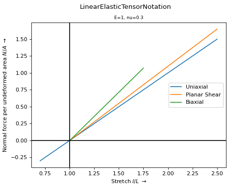
- class felupe.constitution.LinearElasticTensorNotation(E, nu, parallel=False)[ソース]#
Isotropic linear-elastic material formulation.
メモ
\[ \begin{align}\begin{aligned}\boldsymbol{\sigma} &= 2 \mu \ \boldsymbol{\varepsilon} + \gamma \ \text{tr}(\boldsymbol{\varepsilon}) \ \boldsymbol{I}\\\frac{\boldsymbol{\partial \sigma}}{\partial \boldsymbol{\varepsilon}} &= 2 \mu \ \boldsymbol{I} \odot \boldsymbol{I} + \gamma \ \boldsymbol{I} \otimes \boldsymbol{I}\end{aligned}\end{align} \]with the strain tensor
\[\boldsymbol{\varepsilon} = \frac{1}{2} \left( \frac{\partial \boldsymbol{u}} {\partial \boldsymbol{X}} + \left( \frac{\partial \boldsymbol{u}} {\partial \boldsymbol{X}} \right)^T \right)\]サンプル
>>> import felupe as fem
>>>
>>> umat = fem.constitution.LinearElasticTensorNotation(E=1, nu=0.3)
>>> ax = umat.plot()
- copy()#
Return a deep-copy of the constitutive material.
- gradient(x)[ソース]#
Evaluate the stress tensor (as a function of the deformation gradient).
- パラメータ:
x (list of ndarray) -- List with Deformation gradient \(\boldsymbol{F}\) (3x3) as first item.
- 戻り値:
Stress tensor (3x3)
- 戻り値の型:
ndarray
- hessian(x=None, shape=(1, 1), dtype=None)[ソース]#
Evaluate the elasticity tensor. The Deformation gradient is only used for the shape of the trailing axes.
- パラメータ:
- 戻り値:
elasticity tensor (3x3x3x3)
- 戻り値の型:
ndarray
- is_stable(x, hessian=None)#
Return a boolean mask for stability of isotropic material model formulations.
At a given deformation gradient, a normal force is applied on each principal stretch direction. If the resulting incremental stretches are positive, the material model formulation is considered to be stable at the given deformation gradient.
- パラメータ:
x (list of ndarray) -- The list with input arguments. These contain the extracted fields of a
FieldContainer.hessian (ndarray or None, optional) -- Second partial derivative of the strain energy density function w.r.t. the deformation gradient. Default is None.
- 戻り値:
Boolean mask of stability.
- 戻り値の型:
ndarray
メモ
警告
This stability check will lead to a singular matrix for isotropic (hyperelastic) material model formulations without a volumetric part.
サンプル
First, let's check the stability of the Neo-Hookean material model formulation. The stability is evaluated on (valid) principal stretches of a biaxial deformation. All deformations are stable.
>>> import numpy as np
>>> import felupe as fem
>>>
>>> umat = fem.NeoHooke(mu=1.0, bulk=2.0)
>>> view = umat.view()
>>> λ = view.biaxial()[0]
>>>
>>> F = np.zeros((3, 3, 1, λ[0].size))
>>> for a in range(3):
...     F[a, a] = λ[a]
>>>
>>> umat.is_stable([F])
array([[ True,  True,  True,  True,  True,  True,  True,  True,  True,
         True,  True,  True,  True,  True,  True,  True]])
Now, let's check the stability of the Mooney-Rivlin material model formulation. The stability is evaluated on (valid) principal stretches of a biaxial deformation. Biaxial deformations are only stable up to a longitudinal stretch of 1.35.
>>> import numpy as np
>>> import felupe as fem
>>> import felupe.constitution.tensortrax as mat
>>>
>>> umat = fem.Hyperelastic(
...     mat.models.hyperelastic.mooney_rivlin,
...     C10=0.25,
...     C01=0.25,
... ) & fem.Volumetric(bulk=5000)
>>> view = umat.view()
>>> λ = view.biaxial()[0]
>>>
>>> F = np.zeros((3, 3, 1, λ[0].size))
>>> for a in range(3):
...     F[a, a] = λ[a]
>>>
>>> umat.is_stable([F])
array([[ True,  True,  True,  True,  True,  True,  True,  True, False,
        False, False, False, False, False, False, False]])
- optimize(ux=None, ps=None, bx=None, incompressible=False, relative=False, **kwargs)#
Optimize the material parameters by a least-squares fit on experimental stretch-stress data.
- パラメータ:
ux (array of shape (2, ...) or None, optional) -- Experimental uniaxial stretch and force-per-undeformed-area data (default is None).
ps (array of shape (2, ...) or None, optional) -- Experimental planar-shear stretch and force-per-undeformed-area data (default is None).
bx (array of shape (2, ...) or None, optional) -- Experimental biaxial stretch and force-per-undeformed-area data (default is None).
incompressible (bool, optional) -- A flag to enforce incompressible deformations (default is False).
relative (bool, optional) -- A flag to optimize relative instead of absolute residuals, i.e.
(predicted - observed) / observedinstead ofpredicted - observed(default is False).**kwargs (dict, optional) -- Optional keyword arguments are passed to
scipy.optimize.least_squares().
- 戻り値:
ConstitutiveMaterial -- A copy of the constitutive material with the optimized material parameters.
scipy.optimize.OptimizeResult -- Represents the optimization result.
メモ
警告
At least one load case, i.e. one of the arguments
ux,psorbxmust not beNone.注釈
For JAX-based materials, double-precision is required to optimize material parameters.
import jax

jax.config.update("jax_enable_x64", True)
The vector of residuals is given in Eq. (3) in case of absolute residuals
(19)#\[ \begin{align}\begin{aligned}\begin{split}\boldsymbol{r} &= \begin{bmatrix} \boldsymbol{r}_\text{ux} \\ \boldsymbol{r}_\text{ps} \\ \boldsymbol{r}_\text{bx} \end{bmatrix}\end{split}\\r_\text{ux}(\lambda_i) &= P_\text{ux}(\lambda_i) - P_\text{ux, observed}(\lambda_i)\\r_\text{ps}(\lambda_i) &= P_\text{ps}(\lambda_i) - P_\text{ps, observed}(\lambda_i)\\r_\text{bx}(\lambda_i) &= P_\text{bx}(\lambda_i) - P_\text{bx, observed}(\lambda_i)\end{aligned}\end{align} \]and in Eq. (4) in case of relative residuals.
(20)#\[ \begin{align}\begin{aligned}\begin{split}\boldsymbol{r} &= \begin{bmatrix} \boldsymbol{r}_\text{ux} \\ \boldsymbol{r}_\text{ps} \\ \boldsymbol{r}_\text{bx} \end{bmatrix}\end{split}\\r_\text{ux}(\lambda_i) &= \frac{ P_\text{ux}(\lambda_i) - P_\text{ux, observed}(\lambda_i)}{ P_\text{ux, observed}(\lambda_i) }\\r_\text{ps}(\lambda_i) &= \frac{ P_\text{ps}(\lambda_i) - P_\text{ps, observed}(\lambda_i)}{ P_\text{ps, observed}(\lambda_i) }\\r_\text{bx}(\lambda_i) &= \frac{ P_\text{bx}(\lambda_i) - P_\text{bx, observed}(\lambda_i)}{ P_\text{bx, observed}(\lambda_i) }\end{aligned}\end{align} \]サンプル
The
Anssari-Benam Bucchimaterial model formulation is best-fitted on Treloar's uniaxial and biaxial tension data [1]_.>>> import numpy as np >>> import felupe as fem >>> >>> λ, P = np.array( ... [ ... [1.000, 0.00], ... [1.240, 2.30], ... [1.585, 4.16], ... [2.180, 6.00], ... [3.020, 8.80], ... [4.030, 12.5], ... [4.760, 16.2], ... [5.750, 23.6], ... [6.850, 38.5], ... [7.250, 49.6], ... [7.600, 64.4], ... ] ... ).T * np.array([[1.0], [0.0980665]]) >>> >>> umat = fem.Hyperelastic(fem.anssari_benam_bucchi) >>> umat_new, res = umat.optimize( ... ux=[λ, P], incompressible=True, relative=True ... ) >>> >>> ux = np.linspace(λ.min(), λ.max(), num=50) >>> ax = umat_new.plot(incompressible=True, ux=ux, bx=None, ps=None) >>> ax.plot(λ, P, "C0x")

参考
scipy.optimize.least_squaresSolve a nonlinear least-squares problem with bounds on the variables.
参照
- plot(incompressible=False, **kwargs)#
Return a plot with normal force per undeformed area vs. stretch curves for the elementary homogeneous deformations uniaxial tension/compression, planar shear and biaxial tension of a given isotropic material formulation.
- パラメータ:
incompressible (bool, optional) -- A flag to enforce views on incompressible deformations (default is False).
**kwargs (dict, optional) -- Optional keyword-arguments for
ViewMaterialorViewMaterialIncompressible.
- 戻り値の型:
参考
felupe.ViewMaterialCreate views on normal force per undeformed area vs. stretch curves for the elementary homogeneous deformations uniaxial tension/compression, planar shear and biaxial tension of a given isotropic material formulation.
felupe.ViewMaterialIncompressibleCreate views on normal force per undeformed area vs. stretch curves for the elementary homogeneous incompressible deformations uniaxial tension/compression, planar shear and biaxial tension of a given isotropic material formulation.
- screenshot(filename='umat.png', incompressible=False, **kwargs)#
Save a screenshot with normal force per undeformed area vs. stretch curves for the elementary homogeneous deformations uniaxial tension/compression, planar shear and biaxial tension of a given isotropic material formulation.
- パラメータ:
filename (str, optional) -- The filename of the screenshot (default is "umat.png").
incompressible (bool, optional) -- A flag to enforce views on incompressible deformations (default is False).
**kwargs (dict, optional) -- Optional keyword-arguments for
ViewMaterialorViewMaterialIncompressible.
- 戻り値の型:
参考
felupe.ViewMaterialCreate views on normal force per undeformed area vs. stretch curves for the elementary homogeneous deformations uniaxial tension/compression, planar shear and biaxial tension of a given isotropic material formulation.
felupe.ViewMaterialIncompressibleCreate views on normal force per undeformed area vs. stretch curves for the elementary homogeneous incompressible deformations uniaxial tension/compression, planar shear and biaxial tension of a given isotropic material formulation.
- view(incompressible=False, **kwargs)#
Create views on normal force per undeformed area vs. stretch curves for the elementary homogeneous deformations uniaxial tension/compression, planar shear and biaxial tension of a given isotropic material formulation.
- パラメータ:
incompressible (bool, optional) -- A flag to enforce views on incompressible deformations (default is False).
**kwargs (dict, optional) -- Optional keyword-arguments for
ViewMaterialorViewMaterialIncompressible.
- 戻り値の型:
参考
felupe.ViewMaterialCreate views on normal force per undeformed area vs. stretch curves for the elementary homogeneous deformations uniaxial tension/compression, planar shear and biaxial tension of a given isotropic material formulation.
felupe.ViewMaterialIncompressibleCreate views on normal force per undeformed area vs. stretch curves for the elementary homogeneous incompressible deformations uniaxial tension/compression, planar shear and biaxial tension of a given isotropic material formulation.
- class felupe.constitution.LinearElasticPlaneStrain(E, nu)[ソース]#
Plane-strain isotropic linear-elastic material formulation.
メモ
警告
This class must not be used with
FieldPlaneStrainbut withFieldinstead!- gradient(x)[ソース]#
Evaluate the 2d-stress tensor from the deformation gradient.
- パラメータ:
x (list of ndarray) -- List with In-plane components (2x2) of the Deformation gradient \(\boldsymbol{F}\) as first item.
- 戻り値:
In-plane components of stress tensor (2x2)
- 戻り値の型:
ndarray
- hessian(x)[ソース]#
Evaluate the 2d-elasticity tensor from the deformation gradient.
- パラメータ:
x (list of ndarray) -- List with In-plane components (2x2) of the Deformation gradient \(\boldsymbol{F}\) as first item.
- 戻り値:
In-plane components of elasticity tensor (2x2x2x2)
- 戻り値の型:
ndarray
- class felupe.LinearElasticPlaneStress(E, nu)[ソース]#
Plane-stress isotropic linear-elastic material formulation.
- gradient(x)[ソース]#
Evaluate the 2d-stress tensor from the deformation gradient.
- パラメータ:
x (list of ndarray) -- List with In-plane components (2x2) of the Deformation gradient \(\boldsymbol{F}\) as first item.
- 戻り値:
In-plane components of stress tensor (2x2)
- 戻り値の型:
ndarray
- hessian(x=None, shape=(1, 1))[ソース]#
Evaluate the elasticity tensor from the deformation gradient.
- パラメータ:
- 戻り値:
In-plane components of elasticity tensor (2x2x2x2).
- 戻り値の型:
ndarray
- class felupe.LinearElasticPlasticIsotropicHardening(E, nu, sy, K)[ソース]#
Linear-elastic-plastic material formulation with linear isotropic hardening (return mapping algorithm).
- パラメータ:
参考
MaterialStrainA strain-based user-defined material definition with a given function for the stress tensor and the (fourth-order) elasticity tensor.
linear_elastic_plastic_isotropic_hardeningLinear-elastic-plastic material formulation with linear isotropic hardening (return mapping algorithm).
- copy()#
Return a deep-copy of the constitutive material.
- extract(x)#
Extract the input and evaluate strains, stresses and state variables.
- gradient(x)#
- hessian(x)#
- is_stable(x, hessian=None)#
Return a boolean mask for stability of isotropic material model formulations.
At a given deformation gradient, a normal force is applied on each principal stretch direction. If the resulting incremental stretches are positive, the material model formulation is considered to be stable at the given deformation gradient.
- パラメータ:
x (list of ndarray) -- The list with input arguments. These contain the extracted fields of a
FieldContainer.hessian (ndarray or None, optional) -- Second partial derivative of the strain energy density function w.r.t. the deformation gradient. Default is None.
- 戻り値:
Boolean mask of stability.
- 戻り値の型:
ndarray
メモ
警告
This stability check will lead to a singular matrix for isotropic (hyperelastic) material model formulations without a volumetric part.
サンプル
First, let's check the stability of the Neo-Hookean material model formulation. The stability is evaluated on (valid) principal stretches of a biaxial deformation. All deformations are stable.
>>> import numpy as np
>>> import felupe as fem
>>>
>>> umat = fem.NeoHooke(mu=1.0, bulk=2.0)
>>> view = umat.view()
>>> λ = view.biaxial()[0]
>>>
>>> F = np.zeros((3, 3, 1, λ[0].size))
>>> for a in range(3):
...     F[a, a] = λ[a]
>>>
>>> umat.is_stable([F])
array([[ True,  True,  True,  True,  True,  True,  True,  True,  True,
         True,  True,  True,  True,  True,  True,  True]])
Now, let's check the stability of the Mooney-Rivlin material model formulation. The stability is evaluated on (valid) principal stretches of a biaxial deformation. Biaxial deformations are only stable up to a longitudinal stretch of 1.35.
>>> import numpy as np
>>> import felupe as fem
>>> import felupe.constitution.tensortrax as mat
>>>
>>> umat = fem.Hyperelastic(
...     mat.models.hyperelastic.mooney_rivlin,
...     C10=0.25,
...     C01=0.25,
... ) & fem.Volumetric(bulk=5000)
>>> view = umat.view()
>>> λ = view.biaxial()[0]
>>>
>>> F = np.zeros((3, 3, 1, λ[0].size))
>>> for a in range(3):
...     F[a, a] = λ[a]
>>>
>>> umat.is_stable([F])
array([[ True,  True,  True,  True,  True,  True,  True,  True, False,
        False, False, False, False, False, False, False]])
- optimize(ux=None, ps=None, bx=None, incompressible=False, relative=False, **kwargs)#
Optimize the material parameters by a least-squares fit on experimental stretch-stress data.
- パラメータ:
ux (array of shape (2, ...) or None, optional) -- Experimental uniaxial stretch and force-per-undeformed-area data (default is None).
ps (array of shape (2, ...) or None, optional) -- Experimental planar-shear stretch and force-per-undeformed-area data (default is None).
bx (array of shape (2, ...) or None, optional) -- Experimental biaxial stretch and force-per-undeformed-area data (default is None).
incompressible (bool, optional) -- A flag to enforce incompressible deformations (default is False).
relative (bool, optional) -- A flag to optimize relative instead of absolute residuals, i.e.
(predicted - observed) / observedinstead ofpredicted - observed(default is False).**kwargs (dict, optional) -- Optional keyword arguments are passed to
scipy.optimize.least_squares().
- 戻り値:
ConstitutiveMaterial -- A copy of the constitutive material with the optimized material parameters.
scipy.optimize.OptimizeResult -- Represents the optimization result.
メモ
警告
At least one load case, i.e. one of the arguments
ux,psorbxmust not beNone.注釈
For JAX-based materials, double-precision is required to optimize material parameters.
import jax

jax.config.update("jax_enable_x64", True)
The vector of residuals is given in Eq. (3) in case of absolute residuals
(21)#\[ \begin{align}\begin{aligned}\begin{split}\boldsymbol{r} &= \begin{bmatrix} \boldsymbol{r}_\text{ux} \\ \boldsymbol{r}_\text{ps} \\ \boldsymbol{r}_\text{bx} \end{bmatrix}\end{split}\\r_\text{ux}(\lambda_i) &= P_\text{ux}(\lambda_i) - P_\text{ux, observed}(\lambda_i)\\r_\text{ps}(\lambda_i) &= P_\text{ps}(\lambda_i) - P_\text{ps, observed}(\lambda_i)\\r_\text{bx}(\lambda_i) &= P_\text{bx}(\lambda_i) - P_\text{bx, observed}(\lambda_i)\end{aligned}\end{align} \]and in Eq. (4) in case of relative residuals.
(22)#\[ \begin{align}\begin{aligned}\begin{split}\boldsymbol{r} &= \begin{bmatrix} \boldsymbol{r}_\text{ux} \\ \boldsymbol{r}_\text{ps} \\ \boldsymbol{r}_\text{bx} \end{bmatrix}\end{split}\\r_\text{ux}(\lambda_i) &= \frac{ P_\text{ux}(\lambda_i) - P_\text{ux, observed}(\lambda_i)}{ P_\text{ux, observed}(\lambda_i) }\\r_\text{ps}(\lambda_i) &= \frac{ P_\text{ps}(\lambda_i) - P_\text{ps, observed}(\lambda_i)}{ P_\text{ps, observed}(\lambda_i) }\\r_\text{bx}(\lambda_i) &= \frac{ P_\text{bx}(\lambda_i) - P_\text{bx, observed}(\lambda_i)}{ P_\text{bx, observed}(\lambda_i) }\end{aligned}\end{align} \]サンプル
The
Anssari-Benam Bucchimaterial model formulation is best-fitted on Treloar's uniaxial and biaxial tension data [1]_.>>> import numpy as np >>> import felupe as fem >>> >>> λ, P = np.array( ... [ ... [1.000, 0.00], ... [1.240, 2.30], ... [1.585, 4.16], ... [2.180, 6.00], ... [3.020, 8.80], ... [4.030, 12.5], ... [4.760, 16.2], ... [5.750, 23.6], ... [6.850, 38.5], ... [7.250, 49.6], ... [7.600, 64.4], ... ] ... ).T * np.array([[1.0], [0.0980665]]) >>> >>> umat = fem.Hyperelastic(fem.anssari_benam_bucchi) >>> umat_new, res = umat.optimize( ... ux=[λ, P], incompressible=True, relative=True ... ) >>> >>> ux = np.linspace(λ.min(), λ.max(), num=50) >>> ax = umat_new.plot(incompressible=True, ux=ux, bx=None, ps=None) >>> ax.plot(λ, P, "C0x")

参考
scipy.optimize.least_squaresSolve a nonlinear least-squares problem with bounds on the variables.
参照
- plot(incompressible=False, **kwargs)#
Return a plot with normal force per undeformed area vs. stretch curves for the elementary homogeneous deformations uniaxial tension/compression, planar shear and biaxial tension of a given isotropic material formulation.
- パラメータ:
incompressible (bool, optional) -- A flag to enforce views on incompressible deformations (default is False).
**kwargs (dict, optional) -- Optional keyword-arguments for
ViewMaterialorViewMaterialIncompressible.
- 戻り値の型:
参考
felupe.ViewMaterialCreate views on normal force per undeformed area vs. stretch curves for the elementary homogeneous deformations uniaxial tension/compression, planar shear and biaxial tension of a given isotropic material formulation.
felupe.ViewMaterialIncompressibleCreate views on normal force per undeformed area vs. stretch curves for the elementary homogeneous incompressible deformations uniaxial tension/compression, planar shear and biaxial tension of a given isotropic material formulation.
- screenshot(filename='umat.png', incompressible=False, **kwargs)#
Save a screenshot with normal force per undeformed area vs. stretch curves for the elementary homogeneous deformations uniaxial tension/compression, planar shear and biaxial tension of a given isotropic material formulation.
- パラメータ:
filename (str, optional) -- The filename of the screenshot (default is "umat.png").
incompressible (bool, optional) -- A flag to enforce views on incompressible deformations (default is False).
**kwargs (dict, optional) -- Optional keyword-arguments for
ViewMaterialorViewMaterialIncompressible.
- 戻り値の型:
参考
felupe.ViewMaterialCreate views on normal force per undeformed area vs. stretch curves for the elementary homogeneous deformations uniaxial tension/compression, planar shear and biaxial tension of a given isotropic material formulation.
felupe.ViewMaterialIncompressibleCreate views on normal force per undeformed area vs. stretch curves for the elementary homogeneous incompressible deformations uniaxial tension/compression, planar shear and biaxial tension of a given isotropic material formulation.
- view(incompressible=False, **kwargs)#
Create views on normal force per undeformed area vs. stretch curves for the elementary homogeneous deformations uniaxial tension/compression, planar shear and biaxial tension of a given isotropic material formulation.
- パラメータ:
incompressible (bool, optional) -- A flag to enforce views on incompressible deformations (default is False).
**kwargs (dict, optional) -- Optional keyword-arguments for
ViewMaterialorViewMaterialIncompressible.
- 戻り値の型:
参考
felupe.ViewMaterialCreate views on normal force per undeformed area vs. stretch curves for the elementary homogeneous deformations uniaxial tension/compression, planar shear and biaxial tension of a given isotropic material formulation.
felupe.ViewMaterialIncompressibleCreate views on normal force per undeformed area vs. stretch curves for the elementary homogeneous incompressible deformations uniaxial tension/compression, planar shear and biaxial tension of a given isotropic material formulation.
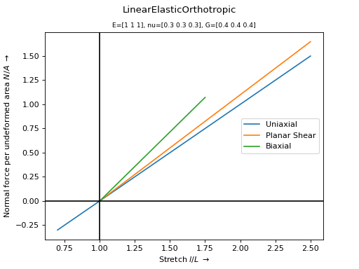
- class felupe.LinearElasticOrthotropic(E, nu, G)[ソース]#
Orthotropic linear-elastic material formulation.
- パラメータ:
サンプル
>>> import felupe as fem
>>>
>>> umat = fem.LinearElasticOrthotropic(
...     E=[1, 1, 1], nu=[0.3, 0.3, 0.3], G=[0.4, 0.4, 0.4]
... )
>>> ax = umat.plot()
- copy()#
Return a deep-copy of the constitutive material.
- gradient(x)[ソース]#
Evaluate the stress tensor (as a function of the deformation gradient).
- パラメータ:
x (list of ndarray) -- List with Deformation gradient \(\boldsymbol{F}\) (3x3) as first item.
- 戻り値:
Stress tensor
- 戻り値の型:
ndarray of shape (3, 3, ...)
- hessian(x=None, shape=(1, 1), dtype=None)[ソース]#
Evaluate the elasticity tensor. The Deformation gradient is only used for the shape of the trailing axes.
- is_stable(x, hessian=None)#
Return a boolean mask for stability of isotropic material model formulations.
At a given deformation gradient, a normal force is applied on each principal stretch direction. If the resulting incremental stretches are positive, the material model formulation is considered to be stable at the given deformation gradient.
- パラメータ:
x (list of ndarray) -- The list with input arguments. These contain the extracted fields of a
FieldContainer.hessian (ndarray or None, optional) -- Second partial derivative of the strain energy density function w.r.t. the deformation gradient. Default is None.
- 戻り値:
Boolean mask of stability.
- 戻り値の型:
ndarray
メモ
警告
This stability check will lead to a singular matrix for isotropic (hyperelastic) material model formulations without a volumetric part.
サンプル
First, let's check the stability of the Neo-Hookean material model formulation. The stability is evaluated on (valid) principal stretches of a biaxial deformation. All deformations are stable.
>>> import numpy as np
>>> import felupe as fem
>>>
>>> umat = fem.NeoHooke(mu=1.0, bulk=2.0)
>>> view = umat.view()
>>> λ = view.biaxial()[0]
>>>
>>> F = np.zeros((3, 3, 1, λ[0].size))
>>> for a in range(3):
...     F[a, a] = λ[a]
>>>
>>> umat.is_stable([F])
array([[ True,  True,  True,  True,  True,  True,  True,  True,  True,
         True,  True,  True,  True,  True,  True,  True]])
Now, let's check the stability of the Mooney-Rivlin material model formulation. The stability is evaluated on (valid) principal stretches of a biaxial deformation. Biaxial deformations are only stable up to a longitudinal stretch of 1.35.
>>> import numpy as np
>>> import felupe as fem
>>> import felupe.constitution.tensortrax as mat
>>>
>>> umat = fem.Hyperelastic(
...     mat.models.hyperelastic.mooney_rivlin,
...     C10=0.25,
...     C01=0.25,
... ) & fem.Volumetric(bulk=5000)
>>> view = umat.view()
>>> λ = view.biaxial()[0]
>>>
>>> F = np.zeros((3, 3, 1, λ[0].size))
>>> for a in range(3):
...     F[a, a] = λ[a]
>>>
>>> umat.is_stable([F])
array([[ True,  True,  True,  True,  True,  True,  True,  True, False,
        False, False, False, False, False, False, False]])
- optimize(ux=None, ps=None, bx=None, incompressible=False, relative=False, **kwargs)#
Optimize the material parameters by a least-squares fit on experimental stretch-stress data.
- パラメータ:
ux (array of shape (2, ...) or None, optional) -- Experimental uniaxial stretch and force-per-undeformed-area data (default is None).
ps (array of shape (2, ...) or None, optional) -- Experimental planar-shear stretch and force-per-undeformed-area data (default is None).
bx (array of shape (2, ...) or None, optional) -- Experimental biaxial stretch and force-per-undeformed-area data (default is None).
incompressible (bool, optional) -- A flag to enforce incompressible deformations (default is False).
relative (bool, optional) -- A flag to optimize relative instead of absolute residuals, i.e.
(predicted - observed) / observedinstead ofpredicted - observed(default is False).**kwargs (dict, optional) -- Optional keyword arguments are passed to
scipy.optimize.least_squares().
- 戻り値:
ConstitutiveMaterial -- A copy of the constitutive material with the optimized material parameters.
scipy.optimize.OptimizeResult -- Represents the optimization result.
メモ
警告
At least one load case, i.e. one of the arguments
ux,psorbxmust not beNone.注釈
For JAX-based materials, double-precision is required to optimize material parameters.
import jax

jax.config.update("jax_enable_x64", True)
The vector of residuals is given in Eq. (3) in case of absolute residuals
(23)#\[ \begin{align}\begin{aligned}\begin{split}\boldsymbol{r} &= \begin{bmatrix} \boldsymbol{r}_\text{ux} \\ \boldsymbol{r}_\text{ps} \\ \boldsymbol{r}_\text{bx} \end{bmatrix}\end{split}\\r_\text{ux}(\lambda_i) &= P_\text{ux}(\lambda_i) - P_\text{ux, observed}(\lambda_i)\\r_\text{ps}(\lambda_i) &= P_\text{ps}(\lambda_i) - P_\text{ps, observed}(\lambda_i)\\r_\text{bx}(\lambda_i) &= P_\text{bx}(\lambda_i) - P_\text{bx, observed}(\lambda_i)\end{aligned}\end{align} \]and in Eq. (4) in case of relative residuals.
(24)#\[ \begin{align}\begin{aligned}\begin{split}\boldsymbol{r} &= \begin{bmatrix} \boldsymbol{r}_\text{ux} \\ \boldsymbol{r}_\text{ps} \\ \boldsymbol{r}_\text{bx} \end{bmatrix}\end{split}\\r_\text{ux}(\lambda_i) &= \frac{ P_\text{ux}(\lambda_i) - P_\text{ux, observed}(\lambda_i)}{ P_\text{ux, observed}(\lambda_i) }\\r_\text{ps}(\lambda_i) &= \frac{ P_\text{ps}(\lambda_i) - P_\text{ps, observed}(\lambda_i)}{ P_\text{ps, observed}(\lambda_i) }\\r_\text{bx}(\lambda_i) &= \frac{ P_\text{bx}(\lambda_i) - P_\text{bx, observed}(\lambda_i)}{ P_\text{bx, observed}(\lambda_i) }\end{aligned}\end{align} \]サンプル
The
Anssari-Benam Bucchimaterial model formulation is best-fitted on Treloar's uniaxial and biaxial tension data [1]_.>>> import numpy as np >>> import felupe as fem >>> >>> λ, P = np.array( ... [ ... [1.000, 0.00], ... [1.240, 2.30], ... [1.585, 4.16], ... [2.180, 6.00], ... [3.020, 8.80], ... [4.030, 12.5], ... [4.760, 16.2], ... [5.750, 23.6], ... [6.850, 38.5], ... [7.250, 49.6], ... [7.600, 64.4], ... ] ... ).T * np.array([[1.0], [0.0980665]]) >>> >>> umat = fem.Hyperelastic(fem.anssari_benam_bucchi) >>> umat_new, res = umat.optimize( ... ux=[λ, P], incompressible=True, relative=True ... ) >>> >>> ux = np.linspace(λ.min(), λ.max(), num=50) >>> ax = umat_new.plot(incompressible=True, ux=ux, bx=None, ps=None) >>> ax.plot(λ, P, "C0x")

参考
scipy.optimize.least_squaresSolve a nonlinear least-squares problem with bounds on the variables.
参照
- plot(incompressible=False, **kwargs)#
Return a plot with normal force per undeformed area vs. stretch curves for the elementary homogeneous deformations uniaxial tension/compression, planar shear and biaxial tension of a given isotropic material formulation.
- パラメータ:
incompressible (bool, optional) -- A flag to enforce views on incompressible deformations (default is False).
**kwargs (dict, optional) -- Optional keyword-arguments for
ViewMaterialorViewMaterialIncompressible.
- 戻り値の型:
参考
felupe.ViewMaterialCreate views on normal force per undeformed area vs. stretch curves for the elementary homogeneous deformations uniaxial tension/compression, planar shear and biaxial tension of a given isotropic material formulation.
felupe.ViewMaterialIncompressibleCreate views on normal force per undeformed area vs. stretch curves for the elementary homogeneous incompressible deformations uniaxial tension/compression, planar shear and biaxial tension of a given isotropic material formulation.
- screenshot(filename='umat.png', incompressible=False, **kwargs)#
Save a screenshot with normal force per undeformed area vs. stretch curves for the elementary homogeneous deformations uniaxial tension/compression, planar shear and biaxial tension of a given isotropic material formulation.
- パラメータ:
filename (str, optional) -- The filename of the screenshot (default is "umat.png").
incompressible (bool, optional) -- A flag to enforce views on incompressible deformations (default is False).
**kwargs (dict, optional) -- Optional keyword-arguments for
ViewMaterialorViewMaterialIncompressible.
- 戻り値の型:
参考
felupe.ViewMaterialCreate views on normal force per undeformed area vs. stretch curves for the elementary homogeneous deformations uniaxial tension/compression, planar shear and biaxial tension of a given isotropic material formulation.
felupe.ViewMaterialIncompressibleCreate views on normal force per undeformed area vs. stretch curves for the elementary homogeneous incompressible deformations uniaxial tension/compression, planar shear and biaxial tension of a given isotropic material formulation.
- view(incompressible=False, **kwargs)#
Create views on normal force per undeformed area vs. stretch curves for the elementary homogeneous deformations uniaxial tension/compression, planar shear and biaxial tension of a given isotropic material formulation.
- パラメータ:
incompressible (bool, optional) -- A flag to enforce views on incompressible deformations (default is False).
**kwargs (dict, optional) -- Optional keyword-arguments for
ViewMaterialorViewMaterialIncompressible.
- 戻り値の型:
参考
felupe.ViewMaterialCreate views on normal force per undeformed area vs. stretch curves for the elementary homogeneous deformations uniaxial tension/compression, planar shear and biaxial tension of a given isotropic material formulation.
felupe.ViewMaterialIncompressibleCreate views on normal force per undeformed area vs. stretch curves for the elementary homogeneous incompressible deformations uniaxial tension/compression, planar shear and biaxial tension of a given isotropic material formulation.
- class felupe.MaterialStrain(material, dim=3, statevars=(0,), framework='small-strain', symmetry=True, **kwargs)[ソース]#
A strain-based user-defined material definition with a given function for the stress tensor and the (fourth-order) elasticity tensor.
- パラメータ:
material (callable) -- The material model formulation. Function signature must be
lambda dε, εn, σn, ζn, **kwargs: dσdε, σ, ζ. Input arguments are the strain increment, old strain, old stress, the list of old state variables and optional keyword arguments. The function must return the algorithmic consistent elasticity tensor, new stress and the list of new state variables. The provided strain and required stress quantities are selected by the framework argument.dim (int, optional) -- The dimension of the material formulation. Default is 3.
statevars (tuple of int, optional) -- A tuple containing the shape of each state variable. Default is (0, ).
framework (str, optional) -- The framework to be used for the stress and strain formulations. "small-strain", "total-lagrange" and "co-rotational" are supported. Default is "small-strain".
symmetry (bool, optional) -- Take the symmetric part of the returned stress and the minor symmetric-parts of the algorithmic consistent elasticity tensor. Default is True. May enhance performance if the material returns symmetric tensors.
メモ
The (default) small-strain framework evaluates the strain tensor as the symmetric part of the displacement gradient, see Eq. (25).
(25)#\[\boldsymbol{\varepsilon} = \operatorname{sym} \left( \frac{\partial \boldsymbol{u}}{\partial \boldsymbol{x}} \right)\]The Total-Lagrange framework uses the Green-Lagrange strain, see Eq. (26),
(26)#\[\boldsymbol{E} = \frac{1}{2} \left( \boldsymbol{C} - \boldsymbol{1} \right)\]with the right Cauchy-Green deformation tensor, as denoted in Eq. (27).
(27)#\[\boldsymbol{C} = \boldsymbol{F}^T \boldsymbol{F}\]Within the Total-Lagrange framework, the second Piola-Kirchhoff stress tensor \(\boldsymbol{S}\), as a function of the Green-Lagrange strain tensor \(\boldsymbol{E}\), is converted to the first Piola-Kirchhoff stress tensor \(\boldsymbol{P}\), see Eq. (28).
(28)#\[\boldsymbol{P} = \boldsymbol{F}\ \boldsymbol{S}\]Furthermore, the fourth-order material elasticity tensor in the Total-Lagrange framework is also converted for algorithmic consistency, see Eq. (29).
(29)#\[\mathbb{A}_{iJkL} = F_{iI}\ F_{kK}\ \mathbb{C}_{IJKL} + \delta_{ik}\ S_{JL}\]警告
The implementation of the co-rotational framework is experimental. The fourth- order elasticity tensor is an approximation and hence, Newton's method does not converge quadratically.
サンプル
Take this code-block for a linear-elastic material formulation
import felupe as fem
from felupe.math import identity, cdya_ik, dya, trace

def linear_elastic(dε, εn, σn, ζn, λ, μ, **kwargs):
    '''3D linear-elastic material formulation.

    Arguments
    ---------
    dε : ndarray
        Incremental strain tensor.
    εn : ndarray
        Old strain tensor.
    σn : ndarray
        Old stress tensor.
    ζn : ndarray
        Old state variables.
    λ : float
        First Lamé-constant.
    μ : float
        Second Lamé-constant (shear modulus).
    '''

    # change of stress due to change of strain
    I = identity(dε)
    dσ = 2 * μ * dε + λ * trace(dε) * I

    # update stress and evaluate elasticity tensor
    σ = σn + dσ
    dσdε = 2 * μ * cdya_ik(I, I) + λ * dya(I, I)

    # update state variables (not used here)
    ζ = ζn

    return dσdε, σ, ζ

umat = fem.MaterialStrain(material=linear_elastic, μ=1, λ=2)
ax = umat.plot()
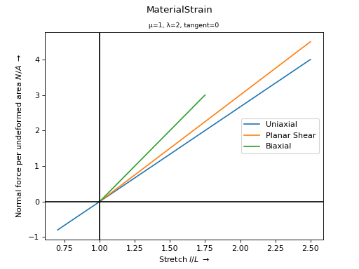
or this minimal header as template.
def fun(dε, εn, σn, ζn, **kwargs):
    return dσdε, σ, ζ

umat = fem.MaterialStrain(material=fun, **kwargs)
The Total-Lagrange framework changes the linear-elastic material formulation to the Saint-Venant Kirchhoff material model formulation.
umat = fem.MaterialStrain(
    material=fem.linear_elastic, μ=1, λ=2, framework="total-lagrange"
)
ax = umat.plot(
    ux=fem.math.linsteps([1, 1.5], num=20),
    ps=fem.math.linsteps([1, 1.5], num=20),
    bx=fem.math.linsteps([1, 1.25], num=10),
)
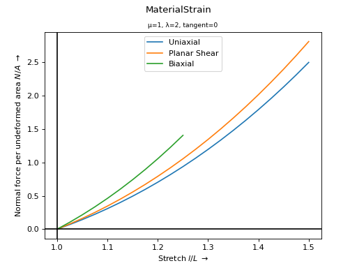
参考
linear_elastic3D linear-elastic material formulation
linear_elastic_plastic_isotropic_hardeningLinear-elastic-plastic material formulation with linear isotropic hardening (return mapping algorithm).
LinearElasticPlasticIsotropicHardeningLinear-elastic-plastic material formulation with linear isotropic hardening (return mapping algorithm).
- copy()#
Return a deep-copy of the constitutive material.
- is_stable(x, hessian=None)#
Return a boolean mask for stability of isotropic material model formulations.
At a given deformation gradient, a normal force is applied on each principal stretch direction. If the resulting incremental stretches are positive, the material model formulation is considered to be stable at the given deformation gradient.
- パラメータ:
x (list of ndarray) -- The list with input arguments. These contain the extracted fields of a
FieldContainer.hessian (ndarray or None, optional) -- Second partial derivative of the strain energy density function w.r.t. the deformation gradient. Default is None.
- 戻り値:
Boolean mask of stability.
- 戻り値の型:
ndarray
メモ
警告
This stability check will lead to a singular matrix for isotropic (hyperelastic) material model formulations without a volumetric part.
サンプル
First, let's check the stability of the Neo-Hookean material model formulation. The stability is evaluated on (valid) principal stretches of a biaxial deformation. All deformations are stable.
>>> import numpy as np
>>> import felupe as fem
>>>
>>> umat = fem.NeoHooke(mu=1.0, bulk=2.0)
>>> view = umat.view()
>>> λ = view.biaxial()[0]
>>>
>>> F = np.zeros((3, 3, 1, λ[0].size))
>>> for a in range(3):
...     F[a, a] = λ[a]
>>>
>>> umat.is_stable([F])
array([[ True,  True,  True,  True,  True,  True,  True,  True,  True,
         True,  True,  True,  True,  True,  True,  True]])
Now, let's check the stability of the Mooney-Rivlin material model formulation. The stability is evaluated on (valid) principal stretches of a biaxial deformation. Biaxial deformations are only stable up to a longitudinal stretch of 1.35.
>>> import numpy as np
>>> import felupe as fem
>>> import felupe.constitution.tensortrax as mat
>>>
>>> umat = fem.Hyperelastic(
...     mat.models.hyperelastic.mooney_rivlin,
...     C10=0.25,
...     C01=0.25,
... ) & fem.Volumetric(bulk=5000)
>>> view = umat.view()
>>> λ = view.biaxial()[0]
>>>
>>> F = np.zeros((3, 3, 1, λ[0].size))
>>> for a in range(3):
...     F[a, a] = λ[a]
>>>
>>> umat.is_stable([F])
array([[ True,  True,  True,  True,  True,  True,  True,  True, False,
        False, False, False, False, False, False, False]])
- optimize(ux=None, ps=None, bx=None, incompressible=False, relative=False, **kwargs)#
Optimize the material parameters by a least-squares fit on experimental stretch-stress data.
- パラメータ:
ux (array of shape (2, ...) or None, optional) -- Experimental uniaxial stretch and force-per-undeformed-area data (default is None).
ps (array of shape (2, ...) or None, optional) -- Experimental planar-shear stretch and force-per-undeformed-area data (default is None).
bx (array of shape (2, ...) or None, optional) -- Experimental biaxial stretch and force-per-undeformed-area data (default is None).
incompressible (bool, optional) -- A flag to enforce incompressible deformations (default is False).
relative (bool, optional) -- A flag to optimize relative instead of absolute residuals, i.e.
(predicted - observed) / observedinstead ofpredicted - observed(default is False).**kwargs (dict, optional) -- Optional keyword arguments are passed to
scipy.optimize.least_squares().
- 戻り値:
ConstitutiveMaterial -- A copy of the constitutive material with the optimized material parameters.
scipy.optimize.OptimizeResult -- Represents the optimization result.
メモ
警告
At least one load case, i.e. one of the arguments
ux,psorbxmust not beNone.注釈
For JAX-based materials, double-precision is required to optimize material parameters.
import jax

jax.config.update("jax_enable_x64", True)
The vector of residuals is given in Eq. (3) in case of absolute residuals
(30)#\[ \begin{align}\begin{aligned}\begin{split}\boldsymbol{r} &= \begin{bmatrix} \boldsymbol{r}_\text{ux} \\ \boldsymbol{r}_\text{ps} \\ \boldsymbol{r}_\text{bx} \end{bmatrix}\end{split}\\r_\text{ux}(\lambda_i) &= P_\text{ux}(\lambda_i) - P_\text{ux, observed}(\lambda_i)\\r_\text{ps}(\lambda_i) &= P_\text{ps}(\lambda_i) - P_\text{ps, observed}(\lambda_i)\\r_\text{bx}(\lambda_i) &= P_\text{bx}(\lambda_i) - P_\text{bx, observed}(\lambda_i)\end{aligned}\end{align} \]and in Eq. (4) in case of relative residuals.
(31)#\[ \begin{align}\begin{aligned}\begin{split}\boldsymbol{r} &= \begin{bmatrix} \boldsymbol{r}_\text{ux} \\ \boldsymbol{r}_\text{ps} \\ \boldsymbol{r}_\text{bx} \end{bmatrix}\end{split}\\r_\text{ux}(\lambda_i) &= \frac{ P_\text{ux}(\lambda_i) - P_\text{ux, observed}(\lambda_i)}{ P_\text{ux, observed}(\lambda_i) }\\r_\text{ps}(\lambda_i) &= \frac{ P_\text{ps}(\lambda_i) - P_\text{ps, observed}(\lambda_i)}{ P_\text{ps, observed}(\lambda_i) }\\r_\text{bx}(\lambda_i) &= \frac{ P_\text{bx}(\lambda_i) - P_\text{bx, observed}(\lambda_i)}{ P_\text{bx, observed}(\lambda_i) }\end{aligned}\end{align} \]サンプル
The
Anssari-Benam Bucchimaterial model formulation is best-fitted on Treloar's uniaxial and biaxial tension data [1]_.>>> import numpy as np >>> import felupe as fem >>> >>> λ, P = np.array( ... [ ... [1.000, 0.00], ... [1.240, 2.30], ... [1.585, 4.16], ... [2.180, 6.00], ... [3.020, 8.80], ... [4.030, 12.5], ... [4.760, 16.2], ... [5.750, 23.6], ... [6.850, 38.5], ... [7.250, 49.6], ... [7.600, 64.4], ... ] ... ).T * np.array([[1.0], [0.0980665]]) >>> >>> umat = fem.Hyperelastic(fem.anssari_benam_bucchi) >>> umat_new, res = umat.optimize( ... ux=[λ, P], incompressible=True, relative=True ... ) >>> >>> ux = np.linspace(λ.min(), λ.max(), num=50) >>> ax = umat_new.plot(incompressible=True, ux=ux, bx=None, ps=None) >>> ax.plot(λ, P, "C0x")

参考
scipy.optimize.least_squaresSolve a nonlinear least-squares problem with bounds on the variables.
参照
- plot(incompressible=False, **kwargs)#
Return a plot with normal force per undeformed area vs. stretch curves for the elementary homogeneous deformations uniaxial tension/compression, planar shear and biaxial tension of a given isotropic material formulation.
- パラメータ:
incompressible (bool, optional) -- A flag to enforce views on incompressible deformations (default is False).
**kwargs (dict, optional) -- Optional keyword-arguments for
ViewMaterialorViewMaterialIncompressible.
- 戻り値の型:
参考
felupe.ViewMaterialCreate views on normal force per undeformed area vs. stretch curves for the elementary homogeneous deformations uniaxial tension/compression, planar shear and biaxial tension of a given isotropic material formulation.
felupe.ViewMaterialIncompressibleCreate views on normal force per undeformed area vs. stretch curves for the elementary homogeneous incompressible deformations uniaxial tension/compression, planar shear and biaxial tension of a given isotropic material formulation.
- screenshot(filename='umat.png', incompressible=False, **kwargs)#
Save a screenshot with normal force per undeformed area vs. stretch curves for the elementary homogeneous deformations uniaxial tension/compression, planar shear and biaxial tension of a given isotropic material formulation.
- パラメータ:
filename (str, optional) -- The filename of the screenshot (default is "umat.png").
incompressible (bool, optional) -- A flag to enforce views on incompressible deformations (default is False).
**kwargs (dict, optional) -- Optional keyword-arguments for
ViewMaterialorViewMaterialIncompressible.
- 戻り値の型:
参考
felupe.ViewMaterialCreate views on normal force per undeformed area vs. stretch curves for the elementary homogeneous deformations uniaxial tension/compression, planar shear and biaxial tension of a given isotropic material formulation.
felupe.ViewMaterialIncompressibleCreate views on normal force per undeformed area vs. stretch curves for the elementary homogeneous incompressible deformations uniaxial tension/compression, planar shear and biaxial tension of a given isotropic material formulation.
- view(incompressible=False, **kwargs)#
Create views on normal force per undeformed area vs. stretch curves for the elementary homogeneous deformations uniaxial tension/compression, planar shear and biaxial tension of a given isotropic material formulation.
- パラメータ:
incompressible (bool, optional) -- A flag to enforce views on incompressible deformations (default is False).
**kwargs (dict, optional) -- Optional keyword-arguments for
ViewMaterialorViewMaterialIncompressible.
- 戻り値の型:
参考
felupe.ViewMaterialCreate views on normal force per undeformed area vs. stretch curves for the elementary homogeneous deformations uniaxial tension/compression, planar shear and biaxial tension of a given isotropic material formulation.
felupe.ViewMaterialIncompressibleCreate views on normal force per undeformed area vs. stretch curves for the elementary homogeneous incompressible deformations uniaxial tension/compression, planar shear and biaxial tension of a given isotropic material formulation.
- class felupe.NearlyIncompressible(material, bulk, parallel=False, dUdJ=<function NearlyIncompressible.<lambda>>, d2UdJdJ=<function NearlyIncompressible.<lambda>>)[ソース]#
A nearly-incompressible material formulation to augment the distortional part of the strain energy function by a volumetric part and a constraint equation.
メモ
The total potential energy of internal forces is given in Eq. (5).
(32)#\[\Pi_{int}(\boldsymbol{F}, p, \bar{J}) = \int_V \hat{\psi}(\boldsymbol{F})\ dV + \int_V U(\bar{J})\ dV + \int_V p (J - \bar{J})\ dV\]The volumetric part of the strain energy density function is denoted in Eq. (9) along with its first and second derivatives.
(33)#\[ \begin{align}\begin{aligned}\bar{U} &= \frac{K}{2} \left( \bar{J} - 1 \right)^2\\\bar{U}' &= K \left( \bar{J} - 1 \right)\\\bar{U}'' &= K\end{aligned}\end{align} \]- パラメータ:
material (ConstitutiveMaterial) -- A hyperelastic material definition for the distortional part of the strain energy density function \(\hat{\psi}(\boldsymbol{F})\) with methods for the
gradient\(\partial_\boldsymbol{F}(\hat{\psi})\) and thehessian\(\partial_\boldsymbol{F}[\partial_\boldsymbol{F}(\hat{\psi})]\) w.r.t the deformation gradient tensor \(\boldsymbol{F}\).bulk (float) -- The bulk modulus \(K\) for the volumetric part of the strain energy function.
parallel (bool, optional) -- A flag to invoke parallel (threaded) math operations (default is False).
dUdJ (callable, optional) -- A function which evaluates the derivative of the volumetric part of the strain energy function \(\bar{U}'\) w.r.t. the volume ratio \(\bar{J}\). Function signature must be
lambda J, bulk: dUdJ. Default is \(\bar{U}' = K (\bar{J} - 1)\) orlambda J, bulk: bulk * (J - 1).d2UdJdJ (callable, optional) -- A function which evaluates the second derivative of the volumetric part of the strain energy function \(\bar{U}''\) w.r.t. the volume ratio \(\bar{J}\). Function signature must be
lambda J, bulk: d2UdJdJ. Default is \(\bar{U}'' = K\) orlambda J, bulk: bulk.
サンプル
>>> import felupe as fem
>>>
>>> field = fem.FieldsMixed(fem.RegionHexahedron(fem.Cube(n=6)), n=3)
>>> boundaries = fem.dof.uniaxial(field, clamped=True, return_loadcase=False)
>>> umat = fem.NearlyIncompressible(fem.NeoHooke(mu=1), bulk=5000)
>>> solid = fem.SolidBody(umat, field)
参考
ThreeFieldVariationHu-Washizu hydrostatic-volumetric selective three-field variation for nearly-incompressible material formulations.
- copy()#
Return a deep-copy of the constitutive material.
- gradient(x, out=None)[ソース]#
Return a list with the gradient of the strain energy density function w.r.t. the fields displacements, pressure and volume ratio.
- パラメータ:
x (list of ndarray) -- List of extracted field values with the deformation gradient tensor \(\boldsymbol{F}\) as first, the pressure \(p\) as second and the volume ratio \(\bar{J}\) as third list item. Initial state variables are stored in the last (fourth) list item.
out (ndarray or None, optional) -- A location into which the result is stored (default is None).
- 戻り値:
List of gradients w.r.t. the input variables \(\boldsymbol{F}\), \(p\) and \(\bar{J}\). The last item of the list contains the updated state variables.
- 戻り値の型:
list of ndarrays
メモ
\[ \begin{align}\begin{aligned}\delta_\boldsymbol{u}(\Pi_{int}) &= \int_V \left( \frac{\partial \hat{\psi}}{\partial \boldsymbol{F}} + p\ J \boldsymbol{F}^{-T} \right) : \delta\boldsymbol{F}\ dV\\\delta_p(\Pi_{int}) &= \int_V \left( J - \bar{J} \right)\ \delta p\ dV\\\delta_\bar{J}(\Pi_{int}) &= \int_V \left( \bar{U}' - p \right)\ \delta \bar{J}\ dV\end{aligned}\end{align} \]
- hessian(x, out=None)[ソース]#
Return a list with the hessian of the strain energy density function w.r.t. the fields displacements, pressure and volume ratio.
- パラメータ:
x (list of ndarray) -- List of extracted field values with the deformation gradient tensor \(\boldsymbol{F}\) as first, the pressure \(p\) as second and the volume ratio \(\bar{J}\) as third list item. Initial state variables are stored in the last (fourth) list item.
out (ndarray or None, optional) -- A location into which the result is stored (default is None).
- 戻り値:
List of the hessian w.r.t. the input variables \(\boldsymbol{F}\), \(p\) and \(\bar{J}\). The upper-triangle items of the hessian are returned as the items of the list.
- 戻り値の型:
list of ndarrays
メモ
\[ \begin{align}\begin{aligned}\Delta_\boldsymbol{u}\delta_\boldsymbol{u}(\Pi_{int}) &= \int_V \delta\boldsymbol{F} : \left[ \frac{\partial^2 \hat{\psi}} {\partial\boldsymbol{F}\ \partial\boldsymbol{F}} + p\ J \left( \boldsymbol{F}^{-T} \otimes \boldsymbol{F}^{-T} - \boldsymbol{F}^{-T} \overset{il}{\odot} \boldsymbol{F}^{-T} \right) \right] : \Delta\boldsymbol{F}\ dV\\\Delta_p\delta_\boldsymbol{u}(\Pi_{int}) &= \int_V \delta\boldsymbol{F} : J \boldsymbol{F}^{-T}\ \Delta p\ dV\\\Delta_\bar{J}\delta_\boldsymbol{u}(\Pi_{int}) &= \int_V \delta\boldsymbol{F} : \boldsymbol{0}\ \Delta \bar{J}\ dV\\\Delta_p\delta_p(\Pi_{int}) &= \int_V \delta p\ (0)\ \Delta p\ dV\\\Delta_p\delta_\bar{J}(\Pi_{int}) &= \int_V \delta \bar{J}\ (-1)\ \Delta p\ dV\\\Delta_\bar{J}\delta_\bar{J}(\Pi_{int}) &= \int_V \delta \bar{J}\ \bar{U}''\ \Delta \bar{J}\ dV\end{aligned}\end{align} \]
- is_stable(x, hessian=None)#
Return a boolean mask for stability of isotropic material model formulations.
At a given deformation gradient, a normal force is applied on each principal stretch direction. If the resulting incremental stretches are positive, the material model formulation is considered to be stable at the given deformation gradient.
- パラメータ:
x (list of ndarray) -- The list with input arguments. These contain the extracted fields of a
FieldContainer.hessian (ndarray or None, optional) -- Second partial derivative of the strain energy density function w.r.t. the deformation gradient. Default is None.
- 戻り値:
Boolean mask of stability.
- 戻り値の型:
ndarray
メモ
警告
This stability check will lead to a singular matrix for isotropic (hyperelastic) material model formulations without a volumetric part.
サンプル
First, let's check the stability of the Neo-Hookean material model formulation. The stability is evaluated on (valid) principal stretches of a biaxial deformation. All deformations are stable.
>>> import numpy as np
>>> import felupe as fem
>>>
>>> umat = fem.NeoHooke(mu=1.0, bulk=2.0)
>>> view = umat.view()
>>> λ = view.biaxial()[0]
>>>
>>> F = np.zeros((3, 3, 1, λ[0].size))
>>> for a in range(3):
...     F[a, a] = λ[a]
>>>
>>> umat.is_stable([F])
array([[ True,  True,  True,  True,  True,  True,  True,  True,  True,
         True,  True,  True,  True,  True,  True,  True]])
Now, let's check the stability of the Mooney-Rivlin material model formulation. The stability is evaluated on (valid) principal stretches of a biaxial deformation. Biaxial deformations are only stable up to a longitudinal stretch of 1.35.
>>> import numpy as np
>>> import felupe as fem
>>> import felupe.constitution.tensortrax as mat
>>>
>>> umat = fem.Hyperelastic(
...     mat.models.hyperelastic.mooney_rivlin,
...     C10=0.25,
...     C01=0.25,
... ) & fem.Volumetric(bulk=5000)
>>> view = umat.view()
>>> λ = view.biaxial()[0]
>>>
>>> F = np.zeros((3, 3, 1, λ[0].size))
>>> for a in range(3):
...     F[a, a] = λ[a]
>>>
>>> umat.is_stable([F])
array([[ True,  True,  True,  True,  True,  True,  True,  True, False,
        False, False, False, False, False, False, False]])
- optimize(ux=None, ps=None, bx=None, incompressible=False, relative=False, **kwargs)#
Optimize the material parameters by a least-squares fit on experimental stretch-stress data.
- パラメータ:
ux (array of shape (2, ...) or None, optional) -- Experimental uniaxial stretch and force-per-undeformed-area data (default is None).
ps (array of shape (2, ...) or None, optional) -- Experimental planar-shear stretch and force-per-undeformed-area data (default is None).
bx (array of shape (2, ...) or None, optional) -- Experimental biaxial stretch and force-per-undeformed-area data (default is None).
incompressible (bool, optional) -- A flag to enforce incompressible deformations (default is False).
relative (bool, optional) -- A flag to optimize relative instead of absolute residuals, i.e.
(predicted - observed) / observedinstead ofpredicted - observed(default is False).**kwargs (dict, optional) -- Optional keyword arguments are passed to
scipy.optimize.least_squares().
- 戻り値:
ConstitutiveMaterial -- A copy of the constitutive material with the optimized material parameters.
scipy.optimize.OptimizeResult -- Represents the optimization result.
メモ
警告
At least one load case, i.e. one of the arguments
ux,psorbxmust not beNone.注釈
For JAX-based materials, double-precision is required to optimize material parameters.
import jax

jax.config.update("jax_enable_x64", True)
The vector of residuals is given in Eq. (3) in case of absolute residuals
(34)#\[ \begin{align}\begin{aligned}\begin{split}\boldsymbol{r} &= \begin{bmatrix} \boldsymbol{r}_\text{ux} \\ \boldsymbol{r}_\text{ps} \\ \boldsymbol{r}_\text{bx} \end{bmatrix}\end{split}\\r_\text{ux}(\lambda_i) &= P_\text{ux}(\lambda_i) - P_\text{ux, observed}(\lambda_i)\\r_\text{ps}(\lambda_i) &= P_\text{ps}(\lambda_i) - P_\text{ps, observed}(\lambda_i)\\r_\text{bx}(\lambda_i) &= P_\text{bx}(\lambda_i) - P_\text{bx, observed}(\lambda_i)\end{aligned}\end{align} \]and in Eq. (4) in case of relative residuals.
(35)#\[ \begin{align}\begin{aligned}\begin{split}\boldsymbol{r} &= \begin{bmatrix} \boldsymbol{r}_\text{ux} \\ \boldsymbol{r}_\text{ps} \\ \boldsymbol{r}_\text{bx} \end{bmatrix}\end{split}\\r_\text{ux}(\lambda_i) &= \frac{ P_\text{ux}(\lambda_i) - P_\text{ux, observed}(\lambda_i)}{ P_\text{ux, observed}(\lambda_i) }\\r_\text{ps}(\lambda_i) &= \frac{ P_\text{ps}(\lambda_i) - P_\text{ps, observed}(\lambda_i)}{ P_\text{ps, observed}(\lambda_i) }\\r_\text{bx}(\lambda_i) &= \frac{ P_\text{bx}(\lambda_i) - P_\text{bx, observed}(\lambda_i)}{ P_\text{bx, observed}(\lambda_i) }\end{aligned}\end{align} \]サンプル
The
Anssari-Benam Bucchimaterial model formulation is best-fitted on Treloar's uniaxial and biaxial tension data [1]_.>>> import numpy as np >>> import felupe as fem >>> >>> λ, P = np.array( ... [ ... [1.000, 0.00], ... [1.240, 2.30], ... [1.585, 4.16], ... [2.180, 6.00], ... [3.020, 8.80], ... [4.030, 12.5], ... [4.760, 16.2], ... [5.750, 23.6], ... [6.850, 38.5], ... [7.250, 49.6], ... [7.600, 64.4], ... ] ... ).T * np.array([[1.0], [0.0980665]]) >>> >>> umat = fem.Hyperelastic(fem.anssari_benam_bucchi) >>> umat_new, res = umat.optimize( ... ux=[λ, P], incompressible=True, relative=True ... ) >>> >>> ux = np.linspace(λ.min(), λ.max(), num=50) >>> ax = umat_new.plot(incompressible=True, ux=ux, bx=None, ps=None) >>> ax.plot(λ, P, "C0x")

参考
scipy.optimize.least_squaresSolve a nonlinear least-squares problem with bounds on the variables.
参照
- plot(incompressible=False, **kwargs)#
Return a plot with normal force per undeformed area vs. stretch curves for the elementary homogeneous deformations uniaxial tension/compression, planar shear and biaxial tension of a given isotropic material formulation.
- パラメータ:
incompressible (bool, optional) -- A flag to enforce views on incompressible deformations (default is False).
**kwargs (dict, optional) -- Optional keyword-arguments for
ViewMaterialorViewMaterialIncompressible.
- 戻り値の型:
参考
felupe.ViewMaterialCreate views on normal force per undeformed area vs. stretch curves for the elementary homogeneous deformations uniaxial tension/compression, planar shear and biaxial tension of a given isotropic material formulation.
felupe.ViewMaterialIncompressibleCreate views on normal force per undeformed area vs. stretch curves for the elementary homogeneous incompressible deformations uniaxial tension/compression, planar shear and biaxial tension of a given isotropic material formulation.
- screenshot(filename='umat.png', incompressible=False, **kwargs)#
Save a screenshot with normal force per undeformed area vs. stretch curves for the elementary homogeneous deformations uniaxial tension/compression, planar shear and biaxial tension of a given isotropic material formulation.
- パラメータ:
filename (str, optional) -- The filename of the screenshot (default is "umat.png").
incompressible (bool, optional) -- A flag to enforce views on incompressible deformations (default is False).
**kwargs (dict, optional) -- Optional keyword-arguments for
ViewMaterialorViewMaterialIncompressible.
- 戻り値の型:
参考
felupe.ViewMaterialCreate views on normal force per undeformed area vs. stretch curves for the elementary homogeneous deformations uniaxial tension/compression, planar shear and biaxial tension of a given isotropic material formulation.
felupe.ViewMaterialIncompressibleCreate views on normal force per undeformed area vs. stretch curves for the elementary homogeneous incompressible deformations uniaxial tension/compression, planar shear and biaxial tension of a given isotropic material formulation.
- view(incompressible=False, **kwargs)#
Create views on normal force per undeformed area vs. stretch curves for the elementary homogeneous deformations uniaxial tension/compression, planar shear and biaxial tension of a given isotropic material formulation.
- パラメータ:
incompressible (bool, optional) -- A flag to enforce views on incompressible deformations (default is False).
**kwargs (dict, optional) -- Optional keyword-arguments for
ViewMaterialorViewMaterialIncompressible.
- 戻り値の型:
参考
felupe.ViewMaterialCreate views on normal force per undeformed area vs. stretch curves for the elementary homogeneous deformations uniaxial tension/compression, planar shear and biaxial tension of a given isotropic material formulation.
felupe.ViewMaterialIncompressibleCreate views on normal force per undeformed area vs. stretch curves for the elementary homogeneous incompressible deformations uniaxial tension/compression, planar shear and biaxial tension of a given isotropic material formulation.
- class felupe.NeoHooke(mu=None, bulk=None, parallel=False)[ソース]#
Nearly-incompressible isotropic hyperelastic Neo-Hookean material formulation. The strain energy density function of the Neo-Hookean material formulation is a linear function of the trace of the isochoric part of the right Cauchy-Green deformation tensor.
- パラメータ:
メモ
注釈
At least one of the two material parameters must not be None.
In a nearly-incompressible constitutive framework the strain energy density is an additive composition of an isochoric and a volumetric part. While the isochoric part is defined on the distortional part of the deformation gradient, the volumetric part of the strain energy function is defined on the determinant of the deformation gradient.
\[ \begin{align}\begin{aligned}\psi &= \hat{\psi}(\hat{\boldsymbol{C}}) + U(J)\\\hat\psi(\hat{\boldsymbol{C}}) &= \frac{\mu}{2} (\text{tr}(\hat{\boldsymbol{C}}) - 3)\end{aligned}\end{align} \]with
\[ \begin{align}\begin{aligned}J &= \text{det}(\boldsymbol{F})\\\hat{\boldsymbol{F}} &= J^{-1/3} \boldsymbol{F}\\\hat{\boldsymbol{C}} &= \hat{\boldsymbol{F}}^T \hat{\boldsymbol{F}}\end{aligned}\end{align} \]The volumetric part of the strain energy density function is a function the volume ratio.
\[U(J) = \frac{K}{2} (J - 1)^2\]The first Piola-Kirchhoff stress tensor is evaluated as the gradient of the strain energy density function. The hessian of the strain energy density function enables the corresponding elasticity tensor.
\[ \begin{align}\begin{aligned}\boldsymbol{P} &= \frac{\partial \psi}{\partial \boldsymbol{F}}\\\mathbb{A} &= \frac{\partial^2 \psi}{\partial \boldsymbol{F}\ \partial \boldsymbol{F}}\end{aligned}\end{align} \]A chain rule application leads to the following expression for the stress tensor. It is formulated as a sum of the physical-deviatoric (not the mathematical deviator!) and the physical-hydrostatic stress tensors.
\[ \begin{align}\begin{aligned}\boldsymbol{P} &= \boldsymbol{P}' + \boldsymbol{P}_U\\\boldsymbol{P}' &= \frac{\partial \hat{\psi}}{\partial \hat{\boldsymbol{F}}} : \frac{\partial \hat{\boldsymbol{F}}}{\partial \boldsymbol{F}} = \bar{\boldsymbol{P}} - \frac{1}{3} (\bar{\boldsymbol{P}} : \boldsymbol{F}) \boldsymbol{F}^{-T}\\\boldsymbol{P}_U &= \frac{\partial U(J)}{\partial J} \frac{\partial J}{\partial \boldsymbol{F}} = U'(J) J \boldsymbol{F}^{-T}\end{aligned}\end{align} \]with
\[ \begin{align}\begin{aligned}\frac{\partial \hat{\boldsymbol{F}}}{\partial \boldsymbol{F}} &= J^{-1/3} \left( \boldsymbol{I} \overset{ik}{\otimes} \boldsymbol{I} - \frac{1}{3} \boldsymbol{F} \otimes \boldsymbol{F}^{-T} \right)\\\frac{\partial J}{\partial \boldsymbol{F}} &= J \boldsymbol{F}^{-T}\\\bar{\boldsymbol{P}} &= J^{-1/3} \frac{\partial \hat{\psi}}{\partial \hat{\boldsymbol{F}}}\end{aligned}\end{align} \]With the above partial derivatives the first Piola-Kirchhoff stress tensor of the Neo-Hookean material model takes the following form.
\[\boldsymbol{P} = \mu J^{-2/3} \left( \boldsymbol{F} - \frac{1}{3} ( \boldsymbol{F} : \boldsymbol{F}) \boldsymbol{F}^{-T} \right) + K (J - 1) J \boldsymbol{F}^{-T}\]Again, a chain rule application leads to an expression for the elasticity tensor.
\[ \begin{align}\begin{aligned}\mathbb{A} &= \mathbb{A}' + \mathbb{A}_{U}\\\mathbb{A}' &= \bar{\mathbb{A}} - \frac{1}{3} \left( (\bar{\mathbb{A}} : \boldsymbol{F}) \otimes \boldsymbol{F}^{-T} + \boldsymbol{F}^{-T} \otimes (\boldsymbol{F} : \bar{\mathbb{A}}) \right ) + \frac{1}{9} (\boldsymbol{F} : \bar{\mathbb{A}} : \boldsymbol{F}) \boldsymbol{F}^{-T} \otimes \boldsymbol{F}^{-T}\\\mathbb{A}_{U} &= (U''(J) J + U'(J)) J \boldsymbol{F}^{-T} \otimes \boldsymbol{F}^{-T} - U'(J) J \boldsymbol{F}^{-T} \overset{il}{\otimes} \boldsymbol{F}^{-T}\end{aligned}\end{align} \]with
\[\bar{\mathbb{A}} = J^{-1/3} \frac{\partial^2 \hat\psi}{\partial \hat{\boldsymbol{F}}\ \partial \hat{\boldsymbol{F}}} J^{-1/3}\]With the above partial derivatives the (physical-deviatoric and -hydrostatic) parts of the elasticity tensor associated to the first Piola-Kirchhoff stress tensor of the Neo-Hookean material model takes the following form.
\[ \begin{align}\begin{aligned}\mathbb{A} &= \mathbb{A}' + \mathbb{A}_{U}\\\mathbb{A}' &= J^{-2/3} \left(\boldsymbol{I} \overset{ik}{\otimes} \boldsymbol{I} - \frac{1}{3} \left( \boldsymbol{F} \otimes \boldsymbol{F}^{-T} + \boldsymbol{F}^{-T} \otimes \boldsymbol{F} \right ) + \frac{1}{9} (\boldsymbol{F} : \boldsymbol{F}) \boldsymbol{F}^{-T} \otimes \boldsymbol{F}^{-T} \right)\\\mathbb{A}_{U} &= K J \left( (2J - 1) \boldsymbol{F}^{-T} \otimes \boldsymbol{F}^{-T} - (J - 1) \boldsymbol{F}^{-T} \overset{il}{\otimes} \boldsymbol{F}^{-T} \right)\end{aligned}\end{align} \]サンプル
>>> import felupe as fem
>>>
>>> umat = fem.NeoHooke(mu=1.0, bulk=2.0)
>>> ax = umat.plot()
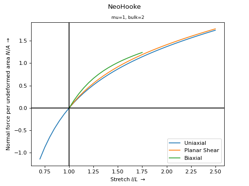
- copy()#
Return a deep-copy of the constitutive material.
- function(x)[ソース]#
Strain energy density function per unit undeformed volume of the Neo-Hookean material formulation.
- パラメータ:
x (list of ndarray) -- List with the Deformation gradient
F(3x3) as first item
- gradient(x, out=None)[ソース]#
Gradient of the strain energy density function per unit undeformed volume of the Neo-Hookean material formulation.
- パラメータ:
x (list of ndarray) -- List with the Deformation gradient
F(3x3) as first itemout (ndarray or None, optional) -- A location into which the result is stored (default is None).
- hessian(x, out=None)[ソース]#
Hessian of the strain energy density function per unit undeformed volume of the Neo-Hookean material formulation.
- パラメータ:
x (list of ndarray) -- List with the Deformation gradient
F(3x3) as first itemout (ndarray or None, optional) -- A location into which the result is stored (default is None).
- is_stable(x, hessian=None)#
Return a boolean mask for stability of isotropic material model formulations.
At a given deformation gradient, a normal force is applied on each principal stretch direction. If the resulting incremental stretches are positive, the material model formulation is considered to be stable at the given deformation gradient.
- パラメータ:
x (list of ndarray) -- The list with input arguments. These contain the extracted fields of a
FieldContainer.hessian (ndarray or None, optional) -- Second partial derivative of the strain energy density function w.r.t. the deformation gradient. Default is None.
- 戻り値:
Boolean mask of stability.
- 戻り値の型:
ndarray
メモ
警告
This stability check will lead to a singular matrix for isotropic (hyperelastic) material model formulations without a volumetric part.
サンプル
First, let's check the stability of the Neo-Hookean material model formulation. The stability is evaluated on (valid) principal stretches of a biaxial deformation. All deformations are stable.
>>> import numpy as np
>>> import felupe as fem
>>>
>>> umat = fem.NeoHooke(mu=1.0, bulk=2.0)
>>> view = umat.view()
>>> λ = view.biaxial()[0]
>>>
>>> F = np.zeros((3, 3, 1, λ[0].size))
>>> for a in range(3):
...     F[a, a] = λ[a]
>>>
>>> umat.is_stable([F])
array([[ True,  True,  True,  True,  True,  True,  True,  True,  True,
         True,  True,  True,  True,  True,  True,  True]])
Now, let's check the stability of the Mooney-Rivlin material model formulation. The stability is evaluated on (valid) principal stretches of a biaxial deformation. Biaxial deformations are only stable up to a longitudinal stretch of 1.35.
>>> import numpy as np
>>> import felupe as fem
>>> import felupe.constitution.tensortrax as mat
>>>
>>> umat = fem.Hyperelastic(
...     mat.models.hyperelastic.mooney_rivlin,
...     C10=0.25,
...     C01=0.25,
... ) & fem.Volumetric(bulk=5000)
>>> view = umat.view()
>>> λ = view.biaxial()[0]
>>>
>>> F = np.zeros((3, 3, 1, λ[0].size))
>>> for a in range(3):
...     F[a, a] = λ[a]
>>>
>>> umat.is_stable([F])
array([[ True,  True,  True,  True,  True,  True,  True,  True, False,
        False, False, False, False, False, False, False]])
- optimize(ux=None, ps=None, bx=None, incompressible=False, relative=False, **kwargs)#
Optimize the material parameters by a least-squares fit on experimental stretch-stress data.
- パラメータ:
ux (array of shape (2, ...) or None, optional) -- Experimental uniaxial stretch and force-per-undeformed-area data (default is None).
ps (array of shape (2, ...) or None, optional) -- Experimental planar-shear stretch and force-per-undeformed-area data (default is None).
bx (array of shape (2, ...) or None, optional) -- Experimental biaxial stretch and force-per-undeformed-area data (default is None).
incompressible (bool, optional) -- A flag to enforce incompressible deformations (default is False).
relative (bool, optional) -- A flag to optimize relative instead of absolute residuals, i.e.
(predicted - observed) / observedinstead ofpredicted - observed(default is False).**kwargs (dict, optional) -- Optional keyword arguments are passed to
scipy.optimize.least_squares().
- 戻り値:
ConstitutiveMaterial -- A copy of the constitutive material with the optimized material parameters.
scipy.optimize.OptimizeResult -- Represents the optimization result.
メモ
警告
At least one load case, i.e. one of the arguments
ux,psorbxmust not beNone.注釈
For JAX-based materials, double-precision is required to optimize material parameters.
import jax

jax.config.update("jax_enable_x64", True)
The vector of residuals is given in Eq. (3) in case of absolute residuals
(36)#\[ \begin{align}\begin{aligned}\begin{split}\boldsymbol{r} &= \begin{bmatrix} \boldsymbol{r}_\text{ux} \\ \boldsymbol{r}_\text{ps} \\ \boldsymbol{r}_\text{bx} \end{bmatrix}\end{split}\\r_\text{ux}(\lambda_i) &= P_\text{ux}(\lambda_i) - P_\text{ux, observed}(\lambda_i)\\r_\text{ps}(\lambda_i) &= P_\text{ps}(\lambda_i) - P_\text{ps, observed}(\lambda_i)\\r_\text{bx}(\lambda_i) &= P_\text{bx}(\lambda_i) - P_\text{bx, observed}(\lambda_i)\end{aligned}\end{align} \]and in Eq. (4) in case of relative residuals.
(37)#\[ \begin{align}\begin{aligned}\begin{split}\boldsymbol{r} &= \begin{bmatrix} \boldsymbol{r}_\text{ux} \\ \boldsymbol{r}_\text{ps} \\ \boldsymbol{r}_\text{bx} \end{bmatrix}\end{split}\\r_\text{ux}(\lambda_i) &= \frac{ P_\text{ux}(\lambda_i) - P_\text{ux, observed}(\lambda_i)}{ P_\text{ux, observed}(\lambda_i) }\\r_\text{ps}(\lambda_i) &= \frac{ P_\text{ps}(\lambda_i) - P_\text{ps, observed}(\lambda_i)}{ P_\text{ps, observed}(\lambda_i) }\\r_\text{bx}(\lambda_i) &= \frac{ P_\text{bx}(\lambda_i) - P_\text{bx, observed}(\lambda_i)}{ P_\text{bx, observed}(\lambda_i) }\end{aligned}\end{align} \]サンプル
The
Anssari-Benam Bucchimaterial model formulation is best-fitted on Treloar's uniaxial and biaxial tension data [1]_.>>> import numpy as np >>> import felupe as fem >>> >>> λ, P = np.array( ... [ ... [1.000, 0.00], ... [1.240, 2.30], ... [1.585, 4.16], ... [2.180, 6.00], ... [3.020, 8.80], ... [4.030, 12.5], ... [4.760, 16.2], ... [5.750, 23.6], ... [6.850, 38.5], ... [7.250, 49.6], ... [7.600, 64.4], ... ] ... ).T * np.array([[1.0], [0.0980665]]) >>> >>> umat = fem.Hyperelastic(fem.anssari_benam_bucchi) >>> umat_new, res = umat.optimize( ... ux=[λ, P], incompressible=True, relative=True ... ) >>> >>> ux = np.linspace(λ.min(), λ.max(), num=50) >>> ax = umat_new.plot(incompressible=True, ux=ux, bx=None, ps=None) >>> ax.plot(λ, P, "C0x")

参考
scipy.optimize.least_squaresSolve a nonlinear least-squares problem with bounds on the variables.
参照
- plot(incompressible=False, **kwargs)#
Return a plot with normal force per undeformed area vs. stretch curves for the elementary homogeneous deformations uniaxial tension/compression, planar shear and biaxial tension of a given isotropic material formulation.
- パラメータ:
incompressible (bool, optional) -- A flag to enforce views on incompressible deformations (default is False).
**kwargs (dict, optional) -- Optional keyword-arguments for
ViewMaterialorViewMaterialIncompressible.
- 戻り値の型:
参考
felupe.ViewMaterialCreate views on normal force per undeformed area vs. stretch curves for the elementary homogeneous deformations uniaxial tension/compression, planar shear and biaxial tension of a given isotropic material formulation.
felupe.ViewMaterialIncompressibleCreate views on normal force per undeformed area vs. stretch curves for the elementary homogeneous incompressible deformations uniaxial tension/compression, planar shear and biaxial tension of a given isotropic material formulation.
- screenshot(filename='umat.png', incompressible=False, **kwargs)#
Save a screenshot with normal force per undeformed area vs. stretch curves for the elementary homogeneous deformations uniaxial tension/compression, planar shear and biaxial tension of a given isotropic material formulation.
- パラメータ:
filename (str, optional) -- The filename of the screenshot (default is "umat.png").
incompressible (bool, optional) -- A flag to enforce views on incompressible deformations (default is False).
**kwargs (dict, optional) -- Optional keyword-arguments for
ViewMaterialorViewMaterialIncompressible.
- 戻り値の型:
参考
felupe.ViewMaterialCreate views on normal force per undeformed area vs. stretch curves for the elementary homogeneous deformations uniaxial tension/compression, planar shear and biaxial tension of a given isotropic material formulation.
felupe.ViewMaterialIncompressibleCreate views on normal force per undeformed area vs. stretch curves for the elementary homogeneous incompressible deformations uniaxial tension/compression, planar shear and biaxial tension of a given isotropic material formulation.
- view(incompressible=False, **kwargs)#
Create views on normal force per undeformed area vs. stretch curves for the elementary homogeneous deformations uniaxial tension/compression, planar shear and biaxial tension of a given isotropic material formulation.
- パラメータ:
incompressible (bool, optional) -- A flag to enforce views on incompressible deformations (default is False).
**kwargs (dict, optional) -- Optional keyword-arguments for
ViewMaterialorViewMaterialIncompressible.
- 戻り値の型:
参考
felupe.ViewMaterialCreate views on normal force per undeformed area vs. stretch curves for the elementary homogeneous deformations uniaxial tension/compression, planar shear and biaxial tension of a given isotropic material formulation.
felupe.ViewMaterialIncompressibleCreate views on normal force per undeformed area vs. stretch curves for the elementary homogeneous incompressible deformations uniaxial tension/compression, planar shear and biaxial tension of a given isotropic material formulation.
- class felupe.NeoHookeCompressible(mu=None, lmbda=None, parallel=False)[ソース]#
Compressible isotropic hyperelastic Neo-Hookean material formulation. The strain energy density function of the Neo-Hookean material formulation is a linear function of the trace of the right Cauchy-Green deformation tensor.
- パラメータ:
メモ
\[ \begin{align}\begin{aligned}\psi &= \psi(\boldsymbol{C})\\\psi(\boldsymbol{C}) &= \frac{\mu}{2} \text{tr}(\boldsymbol{C}) - \mu \ln(J) + \frac{\lambda}{2} \ln(J)^2\end{aligned}\end{align} \]with
\[J = \text{det}(\boldsymbol{F})\]The first Piola-Kirchhoff stress tensor is evaluated as the gradient of the strain energy density function.
\[ \begin{align}\begin{aligned}\boldsymbol{P} &= \frac{\partial \psi}{\partial \boldsymbol{F}}\\\boldsymbol{P} &= \mu \left( \boldsymbol{F} - \boldsymbol{F}^{-T} \right) + \lambda \ln(J) \boldsymbol{F}^{-T}\end{aligned}\end{align} \]The hessian of the strain energy density function enables the corresponding elasticity tensor.
\[ \begin{align}\begin{aligned}\mathbb{A} &= \frac{\partial^2 \psi}{\partial \boldsymbol{F}\ \partial \boldsymbol{F}}\\\mathbb{A} &= \mu \boldsymbol{I} \overset{ik}{\otimes} \boldsymbol{I} + \left(\mu - \lambda \ln(J) \right) \boldsymbol{F}^{-T} \overset{il}{\otimes} \boldsymbol{F}^{-T} + \lambda \boldsymbol{F}^{-T} {\otimes} \boldsymbol{F}^{-T}\end{aligned}\end{align} \]サンプル
>>> import felupe as fem
>>>
>>> umat = fem.NeoHookeCompressible(mu=1.0, lmbda=2.0)
>>> ax = umat.plot()
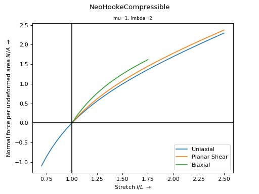
- copy()#
Return a deep-copy of the constitutive material.
- function(x)[ソース]#
Strain energy density function per unit undeformed volume of the Neo-Hookean material formulation.
- パラメータ:
x (list of ndarray) -- List with the Deformation gradient
F(3x3) as first item
- gradient(x, out=None)[ソース]#
Gradient of the strain energy density function per unit undeformed volume of the Neo-Hookean material formulation.
- パラメータ:
x (list of ndarray) -- List with the Deformation gradient
F(3x3) as first itemout (ndarray or None, optional) -- A location into which the result is stored (default is None).
- hessian(x, out=None)[ソース]#
Hessian of the strain energy density function per unit undeformed volume of the Neo-Hookean material formulation.
- パラメータ:
x (list of ndarray) -- List with the Deformation gradient
F(3x3) as first itemout (ndarray or None, optional) -- A location into which the result is stored (default is None).
- is_stable(x, hessian=None)#
Return a boolean mask for stability of isotropic material model formulations.
At a given deformation gradient, a normal force is applied on each principal stretch direction. If the resulting incremental stretches are positive, the material model formulation is considered to be stable at the given deformation gradient.
- パラメータ:
x (list of ndarray) -- The list with input arguments. These contain the extracted fields of a
FieldContainer.hessian (ndarray or None, optional) -- Second partial derivative of the strain energy density function w.r.t. the deformation gradient. Default is None.
- 戻り値:
Boolean mask of stability.
- 戻り値の型:
ndarray
メモ
警告
This stability check will lead to a singular matrix for isotropic (hyperelastic) material model formulations without a volumetric part.
サンプル
First, let's check the stability of the Neo-Hookean material model formulation. The stability is evaluated on (valid) principal stretches of a biaxial deformation. All deformations are stable.
>>> import numpy as np
>>> import felupe as fem
>>>
>>> umat = fem.NeoHooke(mu=1.0, bulk=2.0)
>>> view = umat.view()
>>> λ = view.biaxial()[0]
>>>
>>> F = np.zeros((3, 3, 1, λ[0].size))
>>> for a in range(3):
...     F[a, a] = λ[a]
>>>
>>> umat.is_stable([F])
array([[ True,  True,  True,  True,  True,  True,  True,  True,  True,
         True,  True,  True,  True,  True,  True,  True]])
Now, let's check the stability of the Mooney-Rivlin material model formulation. The stability is evaluated on (valid) principal stretches of a biaxial deformation. Biaxial deformations are only stable up to a longitudinal stretch of 1.35.
>>> import numpy as np
>>> import felupe as fem
>>> import felupe.constitution.tensortrax as mat
>>>
>>> umat = fem.Hyperelastic(
...     mat.models.hyperelastic.mooney_rivlin,
...     C10=0.25,
...     C01=0.25,
... ) & fem.Volumetric(bulk=5000)
>>> view = umat.view()
>>> λ = view.biaxial()[0]
>>>
>>> F = np.zeros((3, 3, 1, λ[0].size))
>>> for a in range(3):
...     F[a, a] = λ[a]
>>>
>>> umat.is_stable([F])
array([[ True,  True,  True,  True,  True,  True,  True,  True, False,
        False, False, False, False, False, False, False]])
- optimize(ux=None, ps=None, bx=None, incompressible=False, relative=False, **kwargs)#
Optimize the material parameters by a least-squares fit on experimental stretch-stress data.
- パラメータ:
ux (array of shape (2, ...) or None, optional) -- Experimental uniaxial stretch and force-per-undeformed-area data (default is None).
ps (array of shape (2, ...) or None, optional) -- Experimental planar-shear stretch and force-per-undeformed-area data (default is None).
bx (array of shape (2, ...) or None, optional) -- Experimental biaxial stretch and force-per-undeformed-area data (default is None).
incompressible (bool, optional) -- A flag to enforce incompressible deformations (default is False).
relative (bool, optional) -- A flag to optimize relative instead of absolute residuals, i.e.
(predicted - observed) / observedinstead ofpredicted - observed(default is False).**kwargs (dict, optional) -- Optional keyword arguments are passed to
scipy.optimize.least_squares().
- 戻り値:
ConstitutiveMaterial -- A copy of the constitutive material with the optimized material parameters.
scipy.optimize.OptimizeResult -- Represents the optimization result.
メモ
警告
At least one load case, i.e. one of the arguments
ux,psorbxmust not beNone.注釈
For JAX-based materials, double-precision is required to optimize material parameters.
import jax

jax.config.update("jax_enable_x64", True)
The vector of residuals is given in Eq. (3) in case of absolute residuals
(38)#\[ \begin{align}\begin{aligned}\begin{split}\boldsymbol{r} &= \begin{bmatrix} \boldsymbol{r}_\text{ux} \\ \boldsymbol{r}_\text{ps} \\ \boldsymbol{r}_\text{bx} \end{bmatrix}\end{split}\\r_\text{ux}(\lambda_i) &= P_\text{ux}(\lambda_i) - P_\text{ux, observed}(\lambda_i)\\r_\text{ps}(\lambda_i) &= P_\text{ps}(\lambda_i) - P_\text{ps, observed}(\lambda_i)\\r_\text{bx}(\lambda_i) &= P_\text{bx}(\lambda_i) - P_\text{bx, observed}(\lambda_i)\end{aligned}\end{align} \]and in Eq. (4) in case of relative residuals.
(39)#\[ \begin{align}\begin{aligned}\begin{split}\boldsymbol{r} &= \begin{bmatrix} \boldsymbol{r}_\text{ux} \\ \boldsymbol{r}_\text{ps} \\ \boldsymbol{r}_\text{bx} \end{bmatrix}\end{split}\\r_\text{ux}(\lambda_i) &= \frac{ P_\text{ux}(\lambda_i) - P_\text{ux, observed}(\lambda_i)}{ P_\text{ux, observed}(\lambda_i) }\\r_\text{ps}(\lambda_i) &= \frac{ P_\text{ps}(\lambda_i) - P_\text{ps, observed}(\lambda_i)}{ P_\text{ps, observed}(\lambda_i) }\\r_\text{bx}(\lambda_i) &= \frac{ P_\text{bx}(\lambda_i) - P_\text{bx, observed}(\lambda_i)}{ P_\text{bx, observed}(\lambda_i) }\end{aligned}\end{align} \]サンプル
The
Anssari-Benam Bucchimaterial model formulation is best-fitted on Treloar's uniaxial and biaxial tension data [1]_.>>> import numpy as np >>> import felupe as fem >>> >>> λ, P = np.array( ... [ ... [1.000, 0.00], ... [1.240, 2.30], ... [1.585, 4.16], ... [2.180, 6.00], ... [3.020, 8.80], ... [4.030, 12.5], ... [4.760, 16.2], ... [5.750, 23.6], ... [6.850, 38.5], ... [7.250, 49.6], ... [7.600, 64.4], ... ] ... ).T * np.array([[1.0], [0.0980665]]) >>> >>> umat = fem.Hyperelastic(fem.anssari_benam_bucchi) >>> umat_new, res = umat.optimize( ... ux=[λ, P], incompressible=True, relative=True ... ) >>> >>> ux = np.linspace(λ.min(), λ.max(), num=50) >>> ax = umat_new.plot(incompressible=True, ux=ux, bx=None, ps=None) >>> ax.plot(λ, P, "C0x")

参考
scipy.optimize.least_squaresSolve a nonlinear least-squares problem with bounds on the variables.
参照
- plot(incompressible=False, **kwargs)#
Return a plot with normal force per undeformed area vs. stretch curves for the elementary homogeneous deformations uniaxial tension/compression, planar shear and biaxial tension of a given isotropic material formulation.
- パラメータ:
incompressible (bool, optional) -- A flag to enforce views on incompressible deformations (default is False).
**kwargs (dict, optional) -- Optional keyword-arguments for
ViewMaterialorViewMaterialIncompressible.
- 戻り値の型:
参考
felupe.ViewMaterialCreate views on normal force per undeformed area vs. stretch curves for the elementary homogeneous deformations uniaxial tension/compression, planar shear and biaxial tension of a given isotropic material formulation.
felupe.ViewMaterialIncompressibleCreate views on normal force per undeformed area vs. stretch curves for the elementary homogeneous incompressible deformations uniaxial tension/compression, planar shear and biaxial tension of a given isotropic material formulation.
- screenshot(filename='umat.png', incompressible=False, **kwargs)#
Save a screenshot with normal force per undeformed area vs. stretch curves for the elementary homogeneous deformations uniaxial tension/compression, planar shear and biaxial tension of a given isotropic material formulation.
- パラメータ:
filename (str, optional) -- The filename of the screenshot (default is "umat.png").
incompressible (bool, optional) -- A flag to enforce views on incompressible deformations (default is False).
**kwargs (dict, optional) -- Optional keyword-arguments for
ViewMaterialorViewMaterialIncompressible.
- 戻り値の型:
参考
felupe.ViewMaterialCreate views on normal force per undeformed area vs. stretch curves for the elementary homogeneous deformations uniaxial tension/compression, planar shear and biaxial tension of a given isotropic material formulation.
felupe.ViewMaterialIncompressibleCreate views on normal force per undeformed area vs. stretch curves for the elementary homogeneous incompressible deformations uniaxial tension/compression, planar shear and biaxial tension of a given isotropic material formulation.
- view(incompressible=False, **kwargs)#
Create views on normal force per undeformed area vs. stretch curves for the elementary homogeneous deformations uniaxial tension/compression, planar shear and biaxial tension of a given isotropic material formulation.
- パラメータ:
incompressible (bool, optional) -- A flag to enforce views on incompressible deformations (default is False).
**kwargs (dict, optional) -- Optional keyword-arguments for
ViewMaterialorViewMaterialIncompressible.
- 戻り値の型:
参考
felupe.ViewMaterialCreate views on normal force per undeformed area vs. stretch curves for the elementary homogeneous deformations uniaxial tension/compression, planar shear and biaxial tension of a given isotropic material formulation.
felupe.ViewMaterialIncompressibleCreate views on normal force per undeformed area vs. stretch curves for the elementary homogeneous incompressible deformations uniaxial tension/compression, planar shear and biaxial tension of a given isotropic material formulation.
- class felupe.OgdenRoxburgh(material, r, m, beta)[ソース]#
Ogden-Roxburgh Pseudo-Elastic material formulation for an isotropic treatment of the load-history dependent Mullins-softening of rubber-like materials.
- パラメータ:
material (NeoHooke, Hyperelastic, Material or MaterialAD) -- An isotropic hyperelastic (user) material definition.
r (float) -- Reciprocal value of the maximum relative amount of softening. i.e.
r=3means the shear modulus of the base material scales down from \(1\) (no softening) to \(1 - 1/3 = 2/3\) (maximum softening).m (float) -- The initial Mullins softening modulus.
beta (float) -- Maximum deformation-dependent part of the Mullins softening modulus.
メモ
\[ \begin{align}\begin{aligned}\eta(\psi, \psi_\text{max}) &= 1 - \frac{1}{r} \text{erf} \left( \frac{\psi_\text{max} - \psi}{m + \beta~\psi_\text{max}} \right)\\\boldsymbol{P} &= \eta \frac{\partial \psi}{\partial \boldsymbol{F}}\\\mathbb{A} &= \frac{\partial^2 \psi}{\partial \boldsymbol{F} \partial \boldsymbol{F}} + \frac{\partial \eta}{\partial \psi} \frac{\partial \psi} {\partial \boldsymbol{F}} \otimes \frac{\partial \psi}{\partial \boldsymbol{F}}\end{aligned}\end{align} \]サンプル
>>> import felupe as fem
>>>
>>> neo_hooke = fem.NeoHooke(mu=1.0)
>>> umat = fem.OgdenRoxburgh(material=neo_hooke, r=3.0, m=1.0, beta=0.0)
>>>
>>> ax = umat.plot(
...     ux=fem.math.linsteps([1, 1.5, 1, 2, 1, 2.5, 1], num=15),
...     ps=None,
...     bx=None,
...     incompressible=True,
... )
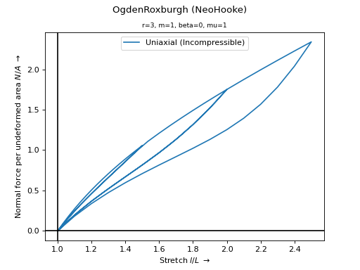
- copy()#
Return a deep-copy of the constitutive material.
- is_stable(x, hessian=None)#
Return a boolean mask for stability of isotropic material model formulations.
At a given deformation gradient, a normal force is applied on each principal stretch direction. If the resulting incremental stretches are positive, the material model formulation is considered to be stable at the given deformation gradient.
- パラメータ:
x (list of ndarray) -- The list with input arguments. These contain the extracted fields of a
FieldContainer.hessian (ndarray or None, optional) -- Second partial derivative of the strain energy density function w.r.t. the deformation gradient. Default is None.
- 戻り値:
Boolean mask of stability.
- 戻り値の型:
ndarray
メモ
警告
This stability check will lead to a singular matrix for isotropic (hyperelastic) material model formulations without a volumetric part.
サンプル
First, let's check the stability of the Neo-Hookean material model formulation. The stability is evaluated on (valid) principal stretches of a biaxial deformation. All deformations are stable.
>>> import numpy as np
>>> import felupe as fem
>>>
>>> umat = fem.NeoHooke(mu=1.0, bulk=2.0)
>>> view = umat.view()
>>> λ = view.biaxial()[0]
>>>
>>> F = np.zeros((3, 3, 1, λ[0].size))
>>> for a in range(3):
...     F[a, a] = λ[a]
>>>
>>> umat.is_stable([F])
array([[ True,  True,  True,  True,  True,  True,  True,  True,  True,
         True,  True,  True,  True,  True,  True,  True]])
Now, let's check the stability of the Mooney-Rivlin material model formulation. The stability is evaluated on (valid) principal stretches of a biaxial deformation. Biaxial deformations are only stable up to a longitudinal stretch of 1.35.
>>> import numpy as np
>>> import felupe as fem
>>> import felupe.constitution.tensortrax as mat
>>>
>>> umat = fem.Hyperelastic(
...     mat.models.hyperelastic.mooney_rivlin,
...     C10=0.25,
...     C01=0.25,
... ) & fem.Volumetric(bulk=5000)
>>> view = umat.view()
>>> λ = view.biaxial()[0]
>>>
>>> F = np.zeros((3, 3, 1, λ[0].size))
>>> for a in range(3):
...     F[a, a] = λ[a]
>>>
>>> umat.is_stable([F])
array([[ True,  True,  True,  True,  True,  True,  True,  True, False,
        False, False, False, False, False, False, False]])
- optimize(ux=None, ps=None, bx=None, incompressible=False, relative=False, **kwargs)#
Optimize the material parameters by a least-squares fit on experimental stretch-stress data.
- パラメータ:
ux (array of shape (2, ...) or None, optional) -- Experimental uniaxial stretch and force-per-undeformed-area data (default is None).
ps (array of shape (2, ...) or None, optional) -- Experimental planar-shear stretch and force-per-undeformed-area data (default is None).
bx (array of shape (2, ...) or None, optional) -- Experimental biaxial stretch and force-per-undeformed-area data (default is None).
incompressible (bool, optional) -- A flag to enforce incompressible deformations (default is False).
relative (bool, optional) -- A flag to optimize relative instead of absolute residuals, i.e.
(predicted - observed) / observedinstead ofpredicted - observed(default is False).**kwargs (dict, optional) -- Optional keyword arguments are passed to
scipy.optimize.least_squares().
- 戻り値:
ConstitutiveMaterial -- A copy of the constitutive material with the optimized material parameters.
scipy.optimize.OptimizeResult -- Represents the optimization result.
メモ
警告
At least one load case, i.e. one of the arguments
ux,psorbxmust not beNone.注釈
For JAX-based materials, double-precision is required to optimize material parameters.
import jax

jax.config.update("jax_enable_x64", True)
The vector of residuals is given in Eq. (3) in case of absolute residuals
(40)#\[ \begin{align}\begin{aligned}\begin{split}\boldsymbol{r} &= \begin{bmatrix} \boldsymbol{r}_\text{ux} \\ \boldsymbol{r}_\text{ps} \\ \boldsymbol{r}_\text{bx} \end{bmatrix}\end{split}\\r_\text{ux}(\lambda_i) &= P_\text{ux}(\lambda_i) - P_\text{ux, observed}(\lambda_i)\\r_\text{ps}(\lambda_i) &= P_\text{ps}(\lambda_i) - P_\text{ps, observed}(\lambda_i)\\r_\text{bx}(\lambda_i) &= P_\text{bx}(\lambda_i) - P_\text{bx, observed}(\lambda_i)\end{aligned}\end{align} \]and in Eq. (4) in case of relative residuals.
(41)#\[ \begin{align}\begin{aligned}\begin{split}\boldsymbol{r} &= \begin{bmatrix} \boldsymbol{r}_\text{ux} \\ \boldsymbol{r}_\text{ps} \\ \boldsymbol{r}_\text{bx} \end{bmatrix}\end{split}\\r_\text{ux}(\lambda_i) &= \frac{ P_\text{ux}(\lambda_i) - P_\text{ux, observed}(\lambda_i)}{ P_\text{ux, observed}(\lambda_i) }\\r_\text{ps}(\lambda_i) &= \frac{ P_\text{ps}(\lambda_i) - P_\text{ps, observed}(\lambda_i)}{ P_\text{ps, observed}(\lambda_i) }\\r_\text{bx}(\lambda_i) &= \frac{ P_\text{bx}(\lambda_i) - P_\text{bx, observed}(\lambda_i)}{ P_\text{bx, observed}(\lambda_i) }\end{aligned}\end{align} \]サンプル
The
Anssari-Benam Bucchimaterial model formulation is best-fitted on Treloar's uniaxial and biaxial tension data [1]_.>>> import numpy as np >>> import felupe as fem >>> >>> λ, P = np.array( ... [ ... [1.000, 0.00], ... [1.240, 2.30], ... [1.585, 4.16], ... [2.180, 6.00], ... [3.020, 8.80], ... [4.030, 12.5], ... [4.760, 16.2], ... [5.750, 23.6], ... [6.850, 38.5], ... [7.250, 49.6], ... [7.600, 64.4], ... ] ... ).T * np.array([[1.0], [0.0980665]]) >>> >>> umat = fem.Hyperelastic(fem.anssari_benam_bucchi) >>> umat_new, res = umat.optimize( ... ux=[λ, P], incompressible=True, relative=True ... ) >>> >>> ux = np.linspace(λ.min(), λ.max(), num=50) >>> ax = umat_new.plot(incompressible=True, ux=ux, bx=None, ps=None) >>> ax.plot(λ, P, "C0x")

参考
scipy.optimize.least_squaresSolve a nonlinear least-squares problem with bounds on the variables.
参照
- plot(incompressible=False, **kwargs)#
Return a plot with normal force per undeformed area vs. stretch curves for the elementary homogeneous deformations uniaxial tension/compression, planar shear and biaxial tension of a given isotropic material formulation.
- パラメータ:
incompressible (bool, optional) -- A flag to enforce views on incompressible deformations (default is False).
**kwargs (dict, optional) -- Optional keyword-arguments for
ViewMaterialorViewMaterialIncompressible.
- 戻り値の型:
参考
felupe.ViewMaterialCreate views on normal force per undeformed area vs. stretch curves for the elementary homogeneous deformations uniaxial tension/compression, planar shear and biaxial tension of a given isotropic material formulation.
felupe.ViewMaterialIncompressibleCreate views on normal force per undeformed area vs. stretch curves for the elementary homogeneous incompressible deformations uniaxial tension/compression, planar shear and biaxial tension of a given isotropic material formulation.
- screenshot(filename='umat.png', incompressible=False, **kwargs)#
Save a screenshot with normal force per undeformed area vs. stretch curves for the elementary homogeneous deformations uniaxial tension/compression, planar shear and biaxial tension of a given isotropic material formulation.
- パラメータ:
filename (str, optional) -- The filename of the screenshot (default is "umat.png").
incompressible (bool, optional) -- A flag to enforce views on incompressible deformations (default is False).
**kwargs (dict, optional) -- Optional keyword-arguments for
ViewMaterialorViewMaterialIncompressible.
- 戻り値の型:
参考
felupe.ViewMaterialCreate views on normal force per undeformed area vs. stretch curves for the elementary homogeneous deformations uniaxial tension/compression, planar shear and biaxial tension of a given isotropic material formulation.
felupe.ViewMaterialIncompressibleCreate views on normal force per undeformed area vs. stretch curves for the elementary homogeneous incompressible deformations uniaxial tension/compression, planar shear and biaxial tension of a given isotropic material formulation.
- view(incompressible=False, **kwargs)#
Create views on normal force per undeformed area vs. stretch curves for the elementary homogeneous deformations uniaxial tension/compression, planar shear and biaxial tension of a given isotropic material formulation.
- パラメータ:
incompressible (bool, optional) -- A flag to enforce views on incompressible deformations (default is False).
**kwargs (dict, optional) -- Optional keyword-arguments for
ViewMaterialorViewMaterialIncompressible.
- 戻り値の型:
参考
felupe.ViewMaterialCreate views on normal force per undeformed area vs. stretch curves for the elementary homogeneous deformations uniaxial tension/compression, planar shear and biaxial tension of a given isotropic material formulation.
felupe.ViewMaterialIncompressibleCreate views on normal force per undeformed area vs. stretch curves for the elementary homogeneous incompressible deformations uniaxial tension/compression, planar shear and biaxial tension of a given isotropic material formulation.
- class felupe.ThreeFieldVariation(material, parallel=False)[ソース]#
Hu-Washizu hydrostatic-volumetric selective \((\boldsymbol{u},p,J)\) - three-field variation for nearly- incompressible material formulations. The total potential energy for nearly-incompressible hyperelasticity is formulated with a determinant-modified deformation gradient. Pressure and volume ratio fields should be kept one order lower than the interpolation order of the displacement field, e.g. linear displacement fields should be paired with element-constant (mean) values of pressure and volume ratio.
The total potential energy of internal forces is defined with a strain energy density function in terms of a determinant-modified deformation gradient and an additional control equation.
\[ \begin{align}\begin{aligned}\Pi &= \Pi_{int} + \Pi_{ext}\\\Pi_{int} &= \int_V \psi(\boldsymbol{F}) \ dV \qquad \rightarrow \qquad \Pi_{int}(\boldsymbol{u},p,J) = \int_V \psi(\overline{\boldsymbol{F}}) \ dV + \int_V p (J-\overline{J}) \ dV\\\overline{\boldsymbol{F}} &= \left(\frac{\overline{J}}{J}\right)^{1/3} \boldsymbol{F}\end{aligned}\end{align} \]The variations of the total potential energy w.r.t. \((\boldsymbol{u},p,J)\) lead to the following expressions. We denote first partial derivatives as \(\boldsymbol{f}_{(\bullet)}\) and second partial derivatives as \(\boldsymbol{A}_{(\bullet,\bullet)}\).
\[ \begin{align}\begin{aligned}\delta_{\boldsymbol{u}} \Pi_{int} &= \int_V \boldsymbol{P} : \delta \boldsymbol{F} \ dV = \int_V \left( \frac{\partial \psi} {\partial \overline{\boldsymbol{F}}} : \frac{\partial \overline{\boldsymbol{F}}} {\partial \boldsymbol{F}} + p J \boldsymbol{F}^{-T} \right) : \delta \boldsymbol{F} \ dV\\\delta_{p} \Pi_{int} &= \int_V f_{p} \ \delta p \ dV = \int_V (J - \overline{J}) \ \delta p \ dV\\\delta_{\overline{J}} \Pi_{int} &= \int_V f_{\overline{J}} \ \delta \overline{J} \ dV = \int_V \left( \frac{\partial \psi}{\partial \overline{\boldsymbol{F}}} : \frac{\partial \overline{\boldsymbol{F}}}{\partial \overline{J}} - p \right) : \delta \overline{J} \ dV\end{aligned}\end{align} \]The projection tensors from the variations lead the following results.
\[ \begin{align}\begin{aligned}\frac{\partial \overline{\boldsymbol{F}}}{\partial \boldsymbol{F}} &= \left(\frac{\overline{J}}{J}\right)^{1/3} \left( \boldsymbol{I} \overset{ik}{\odot} \boldsymbol{I} - \frac{1}{3} \boldsymbol{F} \otimes \boldsymbol{F}^{-T} \right)\\\frac{\partial \overline{\boldsymbol{F}}}{\partial \overline{J}} &= \frac{1}{3 \overline{J}} \overline{\boldsymbol{F}}\end{aligned}\end{align} \]The double-dot products from the variations are now evaluated.
\[ \begin{align}\begin{aligned}\overline{\boldsymbol{P}} &= \frac{\partial \psi}{\partial \overline{\boldsymbol{F}}} = \overline{\overline{\boldsymbol{P}}} - \frac{1}{3} \left( \overline{\overline{\boldsymbol{P}}} : \boldsymbol{F} \right) \boldsymbol{F}^{-T} \qquad \text{with} \qquad \overline{\overline{\boldsymbol{P}}} = \left(\frac{\overline{J}}{J}\right)^{1/3} \frac{\partial \psi}{\partial \overline{\boldsymbol{F}}}\\\frac{\partial \psi}{\partial \overline{\boldsymbol{F}}} : \frac{1}{3 \overline{J}} \overline{\boldsymbol{F}} &= \frac{1}{3 \overline{J}} \overline{\overline{\boldsymbol{P}}} : \boldsymbol{F}\end{aligned}\end{align} \]We now have three formulas; one for the first Piola Kirchhoff stress and two additional control equations.
\[ \begin{align}\begin{aligned}\boldsymbol{P} &= \overline{\overline{\boldsymbol{P}}} - \frac{1}{3} \left( \overline{\overline{\boldsymbol{P}}} : \boldsymbol{F} \right) \boldsymbol{F}^{-T}\\f_p &= J - \overline{J}\\f_{\overline{J}} &= \frac{1}{3 \overline{J}} \left( \overline{\overline{\boldsymbol{P}}} : \boldsymbol{F} \right) - p\end{aligned}\end{align} \]A linearization of the above formulas gives six equations (only results are given here).
\[ \begin{align}\begin{aligned}\mathbb{A}_{\boldsymbol{u},\boldsymbol{u}} &= \overline{\overline{\mathbb{A}}} + \frac{1}{9} \left( \boldsymbol{F} : \overline{\overline{\mathbb{A}}} : \boldsymbol{F} \right) \boldsymbol{F}^{-T} \otimes \boldsymbol{F}^{-T} - \frac{1}{3} \left( \boldsymbol{F}^{-T} \otimes \left( \overline{\overline{\boldsymbol{P}}} + \boldsymbol{F} : \overline{\overline{\mathbb{A}}} \right) + \left( \overline{\overline{\boldsymbol{P}}} + \overline{\overline{\mathbb{A}}} : \boldsymbol{F} \right) \otimes \boldsymbol{F}^{-T} \right)\\&+\left( p J + \frac{1}{9} \overline{\overline{\boldsymbol{P}}} : \boldsymbol{F} \right) \boldsymbol{F}^{-T} \otimes \boldsymbol{F}^{-T} - \left( p J - \frac{1}{3} \overline{\overline{\boldsymbol{P}}} : \boldsymbol{F} \right) \boldsymbol{F}^{-T} \overset{il}{\odot} \boldsymbol{F}^{-T}\\A_{p,p} &= 0\\A_{\overline{J},\overline{J}} &= \frac{1}{9 \overline{J}^2} \left( \boldsymbol{F} : \overline{\overline{\mathbb{A}}} : \boldsymbol{F} \right) - 2 \left( \overline{\overline{\boldsymbol{P}}} : \boldsymbol{F} \right)\\\boldsymbol{A}_{\boldsymbol{u},p} &= \boldsymbol{A}_{p, \boldsymbol{u}} = J \boldsymbol{F}^{-T}\\\boldsymbol{A}_{\boldsymbol{u},\overline{J}} &= \boldsymbol{A}_{\overline{J}, \boldsymbol{u}} = \frac{1}{3 \overline{J}} \left( \boldsymbol{P}' + \boldsymbol{F} : \overline{\overline{\mathbb{A}}} - \frac{1}{3} \left( \boldsymbol{F} : \overline{\overline{\mathbb{A}}} : \boldsymbol{F} \right) \boldsymbol{F}^{-T} \right)\\A_{p,\overline{J}} &= A_{\overline{J}, p} = -1\end{aligned}\end{align} \]with
\[\overline{\overline{\mathbb{A}}} = \left(\frac{\overline{J}}{J}\right)^{1/3} \frac{\partial^2 \psi}{\partial \overline{\boldsymbol{F}} \partial \overline{\boldsymbol{F}}} \left(\frac{\overline{J}}{J}\right)^{1/3}\]as well as
\[\boldsymbol{P}' = \boldsymbol{P} - p J \boldsymbol{F}^{-T}\]- パラメータ:
material (ConstitutiveMaterial) -- A hyperelastic material definition for the strain energy density function with methods for the
gradientand thehessianw.r.t the deformation gradient tensor.parallel (bool, optional) -- A flag to invoke parallel (threaded) math operations (default is False).
- copy()#
Return a deep-copy of the constitutive material.
- gradient(x)[ソース]#
Return a list of variations of the total potential energy w.r.t. the fields displacements, pressure and volume ratio.
- パラメータ:
x (list of ndarray) -- List of extracted field values with the Deformation gradient tensor \(\boldsymbol{F}\) as first, the hydrostatic pressure \(p\) as second and the volume ratio \(\bar{J}\) as third list item.
- 戻り値:
List of gradients w.r.t. the input variables \(\boldsymbol{F}\), \(p\) and \(\bar{J}\).
- 戻り値の型:
list of ndarrays
- hessian(x)[ソース]#
List of linearized variations of total potential energy w.r.t displacements, pressure and volume ratio (these expressions are symmetric;
A_up = A_puif derived from a total potential energy formulation). List entries have to be arranged as a flattened list from the upper triangle blocks:Δ_u(δ_u(Π_int)) = ∫_V δF : (∂²ψ/(∂F∂F) + p ∂cof(F)/∂F) : ΔF dV Δ_p(δ_u(Π_int)) = ∫_V δF : J cof(F) Δp dV Δ_J(δ_u(Π_int)) = ∫_V δF : ∂²ψ/(∂F∂J) ΔJ dV Δ_p(δ_p(Π_int)) = ∫_V δp 0 Δp dV Δ_J(δ_p(Π_int)) = ∫_V δp (-1) ΔJ dV Δ_J(δ_J(Π_int)) = ∫_V δJ ∂²ψ/(∂J∂J) ΔJ dV [[0 1 2], [ 3 4], [ 5]] --> [0 1 2 3 4 5]
- is_stable(x, hessian=None)#
Return a boolean mask for stability of isotropic material model formulations.
At a given deformation gradient, a normal force is applied on each principal stretch direction. If the resulting incremental stretches are positive, the material model formulation is considered to be stable at the given deformation gradient.
- パラメータ:
x (list of ndarray) -- The list with input arguments. These contain the extracted fields of a
FieldContainer.hessian (ndarray or None, optional) -- Second partial derivative of the strain energy density function w.r.t. the deformation gradient. Default is None.
- 戻り値:
Boolean mask of stability.
- 戻り値の型:
ndarray
メモ
警告
This stability check will lead to a singular matrix for isotropic (hyperelastic) material model formulations without a volumetric part.
サンプル
First, let's check the stability of the Neo-Hookean material model formulation. The stability is evaluated on (valid) principal stretches of a biaxial deformation. All deformations are stable.
>>> import numpy as np
>>> import felupe as fem
>>>
>>> umat = fem.NeoHooke(mu=1.0, bulk=2.0)
>>> view = umat.view()
>>> λ = view.biaxial()[0]
>>>
>>> F = np.zeros((3, 3, 1, λ[0].size))
>>> for a in range(3):
...     F[a, a] = λ[a]
>>>
>>> umat.is_stable([F])
array([[ True,  True,  True,  True,  True,  True,  True,  True,  True,
         True,  True,  True,  True,  True,  True,  True]])
Now, let's check the stability of the Mooney-Rivlin material model formulation. The stability is evaluated on (valid) principal stretches of a biaxial deformation. Biaxial deformations are only stable up to a longitudinal stretch of 1.35.
>>> import numpy as np
>>> import felupe as fem
>>> import felupe.constitution.tensortrax as mat
>>>
>>> umat = fem.Hyperelastic(
...     mat.models.hyperelastic.mooney_rivlin,
...     C10=0.25,
...     C01=0.25,
... ) & fem.Volumetric(bulk=5000)
>>> view = umat.view()
>>> λ = view.biaxial()[0]
>>>
>>> F = np.zeros((3, 3, 1, λ[0].size))
>>> for a in range(3):
...     F[a, a] = λ[a]
>>>
>>> umat.is_stable([F])
array([[ True,  True,  True,  True,  True,  True,  True,  True, False,
        False, False, False, False, False, False, False]])
- optimize(ux=None, ps=None, bx=None, incompressible=False, relative=False, **kwargs)#
Optimize the material parameters by a least-squares fit on experimental stretch-stress data.
- パラメータ:
ux (array of shape (2, ...) or None, optional) -- Experimental uniaxial stretch and force-per-undeformed-area data (default is None).
ps (array of shape (2, ...) or None, optional) -- Experimental planar-shear stretch and force-per-undeformed-area data (default is None).
bx (array of shape (2, ...) or None, optional) -- Experimental biaxial stretch and force-per-undeformed-area data (default is None).
incompressible (bool, optional) -- A flag to enforce incompressible deformations (default is False).
relative (bool, optional) -- A flag to optimize relative instead of absolute residuals, i.e.
(predicted - observed) / observedinstead ofpredicted - observed(default is False).**kwargs (dict, optional) -- Optional keyword arguments are passed to
scipy.optimize.least_squares().
- 戻り値:
ConstitutiveMaterial -- A copy of the constitutive material with the optimized material parameters.
scipy.optimize.OptimizeResult -- Represents the optimization result.
メモ
警告
At least one load case, i.e. one of the arguments
ux,psorbxmust not beNone.注釈
For JAX-based materials, double-precision is required to optimize material parameters.
import jax

jax.config.update("jax_enable_x64", True)
The vector of residuals is given in Eq. (3) in case of absolute residuals
(42)#\[ \begin{align}\begin{aligned}\begin{split}\boldsymbol{r} &= \begin{bmatrix} \boldsymbol{r}_\text{ux} \\ \boldsymbol{r}_\text{ps} \\ \boldsymbol{r}_\text{bx} \end{bmatrix}\end{split}\\r_\text{ux}(\lambda_i) &= P_\text{ux}(\lambda_i) - P_\text{ux, observed}(\lambda_i)\\r_\text{ps}(\lambda_i) &= P_\text{ps}(\lambda_i) - P_\text{ps, observed}(\lambda_i)\\r_\text{bx}(\lambda_i) &= P_\text{bx}(\lambda_i) - P_\text{bx, observed}(\lambda_i)\end{aligned}\end{align} \]and in Eq. (4) in case of relative residuals.
(43)#\[ \begin{align}\begin{aligned}\begin{split}\boldsymbol{r} &= \begin{bmatrix} \boldsymbol{r}_\text{ux} \\ \boldsymbol{r}_\text{ps} \\ \boldsymbol{r}_\text{bx} \end{bmatrix}\end{split}\\r_\text{ux}(\lambda_i) &= \frac{ P_\text{ux}(\lambda_i) - P_\text{ux, observed}(\lambda_i)}{ P_\text{ux, observed}(\lambda_i) }\\r_\text{ps}(\lambda_i) &= \frac{ P_\text{ps}(\lambda_i) - P_\text{ps, observed}(\lambda_i)}{ P_\text{ps, observed}(\lambda_i) }\\r_\text{bx}(\lambda_i) &= \frac{ P_\text{bx}(\lambda_i) - P_\text{bx, observed}(\lambda_i)}{ P_\text{bx, observed}(\lambda_i) }\end{aligned}\end{align} \]サンプル
The
Anssari-Benam Bucchimaterial model formulation is best-fitted on Treloar's uniaxial and biaxial tension data [1]_.>>> import numpy as np >>> import felupe as fem >>> >>> λ, P = np.array( ... [ ... [1.000, 0.00], ... [1.240, 2.30], ... [1.585, 4.16], ... [2.180, 6.00], ... [3.020, 8.80], ... [4.030, 12.5], ... [4.760, 16.2], ... [5.750, 23.6], ... [6.850, 38.5], ... [7.250, 49.6], ... [7.600, 64.4], ... ] ... ).T * np.array([[1.0], [0.0980665]]) >>> >>> umat = fem.Hyperelastic(fem.anssari_benam_bucchi) >>> umat_new, res = umat.optimize( ... ux=[λ, P], incompressible=True, relative=True ... ) >>> >>> ux = np.linspace(λ.min(), λ.max(), num=50) >>> ax = umat_new.plot(incompressible=True, ux=ux, bx=None, ps=None) >>> ax.plot(λ, P, "C0x")

参考
scipy.optimize.least_squaresSolve a nonlinear least-squares problem with bounds on the variables.
参照
- plot(incompressible=False, **kwargs)#
Return a plot with normal force per undeformed area vs. stretch curves for the elementary homogeneous deformations uniaxial tension/compression, planar shear and biaxial tension of a given isotropic material formulation.
- パラメータ:
incompressible (bool, optional) -- A flag to enforce views on incompressible deformations (default is False).
**kwargs (dict, optional) -- Optional keyword-arguments for
ViewMaterialorViewMaterialIncompressible.
- 戻り値の型:
参考
felupe.ViewMaterialCreate views on normal force per undeformed area vs. stretch curves for the elementary homogeneous deformations uniaxial tension/compression, planar shear and biaxial tension of a given isotropic material formulation.
felupe.ViewMaterialIncompressibleCreate views on normal force per undeformed area vs. stretch curves for the elementary homogeneous incompressible deformations uniaxial tension/compression, planar shear and biaxial tension of a given isotropic material formulation.
- screenshot(filename='umat.png', incompressible=False, **kwargs)#
Save a screenshot with normal force per undeformed area vs. stretch curves for the elementary homogeneous deformations uniaxial tension/compression, planar shear and biaxial tension of a given isotropic material formulation.
- パラメータ:
filename (str, optional) -- The filename of the screenshot (default is "umat.png").
incompressible (bool, optional) -- A flag to enforce views on incompressible deformations (default is False).
**kwargs (dict, optional) -- Optional keyword-arguments for
ViewMaterialorViewMaterialIncompressible.
- 戻り値の型:
参考
felupe.ViewMaterialCreate views on normal force per undeformed area vs. stretch curves for the elementary homogeneous deformations uniaxial tension/compression, planar shear and biaxial tension of a given isotropic material formulation.
felupe.ViewMaterialIncompressibleCreate views on normal force per undeformed area vs. stretch curves for the elementary homogeneous incompressible deformations uniaxial tension/compression, planar shear and biaxial tension of a given isotropic material formulation.
- view(incompressible=False, **kwargs)#
Create views on normal force per undeformed area vs. stretch curves for the elementary homogeneous deformations uniaxial tension/compression, planar shear and biaxial tension of a given isotropic material formulation.
- パラメータ:
incompressible (bool, optional) -- A flag to enforce views on incompressible deformations (default is False).
**kwargs (dict, optional) -- Optional keyword-arguments for
ViewMaterialorViewMaterialIncompressible.
- 戻り値の型:
参考
felupe.ViewMaterialCreate views on normal force per undeformed area vs. stretch curves for the elementary homogeneous deformations uniaxial tension/compression, planar shear and biaxial tension of a given isotropic material formulation.
felupe.ViewMaterialIncompressibleCreate views on normal force per undeformed area vs. stretch curves for the elementary homogeneous incompressible deformations uniaxial tension/compression, planar shear and biaxial tension of a given isotropic material formulation.