Materials with Automatic Differentiation (tensortrax)#

This page contains hyperelastic material model formulations with automatic differentiation using tensortrax.math.

Frameworks

`Hyperelastic`(fun[, nstatevars, parallel])	A hyperelastic material definition with a given function for the strain energy density function per unit undeformed volume with Automatic Differentiation provided by `tensortrax`.
`Material`(fun[, nstatevars, parallel])	A material definition with a given function for the partial derivative of the strain energy function w.r.t.
`total_lagrange`(material)	Decorate a second Piola-Kirchhoff stress Total-Lagrange material formulation as a first Piola-Kirchoff stress function.
`updated_lagrange`(material)	Decorate a Cauchy-stress Updated-Lagrange material formulation as a first Piola- Kirchoff stress function.

Material Models for felupe.constitution.tensortrax.Hyperelastic

These material model formulations are defined by a strain energy density function.

`alexander`(C, C1, C2, C3, gamma, k)	Strain energy function of the isotropic hyperelastic Alexander material formulation [1]_.
`anssari_benam_bucchi`(C, mu, N)	Strain energy function of the isotropic hyperelastic generalized Neo-Hookean Anssari-Benam Bucchi material formulation [1]_.
`arruda_boyce`(C, C1, limit)	Strain energy function of the isotropic hyperelastic Arruda-Boyce material formulation.
`blatz_ko`(C, mu)	Strain energy function of the Blatz-Ko isotropic hyperelastic foam material formulation [1]_.
`extended_tube`(C, Gc, delta, Ge, beta)	Strain energy function of the isotropic hyperelastic Extended Tube [1]_ material formulation.
`finite_strain_viscoelastic`(C, Cin, mu, eta, ...)	Multiplicative finite strain viscoelastic [1]_ material formulation.
`lopez_pamies`(C, mu, alpha)	Strain energy function of the isotropic hyperelastic Lopez-Pamies material formulation [1]_.
`miehe_goektepe_lulei`(C, mu, N, U, p, q)	Strain energy function of the isotropic hyperelastic micro-sphere model formulation [1]_.
`mooney_rivlin`(C, C10, C01)	Strain energy function of the isotropic hyperelastic Mooney-Rivlin material formulation.
`neo_hooke`(C, mu)	Strain energy function of the isotropic hyperelastic Neo-Hookean material formulation.
`ogden`(C, mu, alpha)	Strain energy function of the isotropic hyperelastic Ogden material formulation.
`ogden_roxburgh`(C, Wmax_n, material, r, m, ...)	Ogden-Roxburgh Pseudo-Elastic material formulation for an isotropic treatment of the load-history dependent Mullins-softening of rubber-like materials.
`saint_venant_kirchhoff`(C, mu, lmbda[, k])	Strain energy function of the isotropic hyperelastic Saint-Venant Kirchhoff material formulation.
`saint_venant_kirchhoff_orthotropic`(C, mu, ...)	Strain energy function of the orthotropic hyperelastic Saint-Venant Kirchhoff material formulation.
`storakers`(C, mu, alpha, beta)	Strain energy function of the Storåkers isotropic hyperelastic foam material formulation [1]_.
`third_order_deformation`(C, C10, C01, C11, ...)	Strain energy function of the isotropic hyperelastic Third-Order-Deformation material formulation.
`van_der_waals`(C, mu, limit, a, beta)	Strain energy function of the Van der Waals [1]_ material formulation.
`yeoh`(C, C10, C20, C30)	Strain energy function of the isotropic hyperelastic Yeoh material formulation.

Material Models for felupe.constitution.tensortrax.Material

The material model formulations are defined by the first Piola-Kirchhoff stress tensor. Function-decorators are available to use total_lagrange() and updated_lagrange() material formulations in Material.

`becker`(F, mu, lmbda)	Second Piola-Kirchhoff stress tensor of Becker's logarithmic material model formulation [1]_ [2]_.
`morph`(F, statevars, p)	Second Piola-Kirchhoff stress tensor of the MORPH model formulation [1]_.
`morph_representative_directions`(F, ...)	First Piola-Kirchhoff stress tensor of the MORPH model formulation [1]_, implemented by the concept of representative directions [2]_, [3].

Detailed API Reference

class felupe.constitution.tensortrax.Hyperelastic(fun, nstatevars=0, parallel=False, **kwargs)[ソース]#

A hyperelastic material definition with a given function for the strain energy density function per unit undeformed volume with Automatic Differentiation provided by tensortrax.

パラメータ:

fun (callable) -- A strain energy density function in terms of the right Cauchy-Green deformation tensor \(\boldsymbol{C}\). Function signature must be fun = lambda C, **kwargs: psi for functions without state variables and fun = lambda C, statevars, **kwargs: [psi, statevars_new] for functions with state variables. The right Cauchy-Green deformation tensor will be a tensortrax.Tensor when the function is evaluated. It is important to use only differentiable math-functions from tensortrax.math.
nstatevars (int, optional) -- Number of state variables (default is 0).
parallel (bool, optional) -- A flag to invoke threaded strain energy density function evaluations (default is False). May introduce additional overhead for small-sized problems.
**kwargs (dict, optional) -- Optional keyword-arguments for the strain energy density function.

メモ

The strain energy density function \(\psi\) must be given in terms of the right Cauchy-Green deformation tensor \(\boldsymbol{C} = \boldsymbol{F}^T \boldsymbol{F}\).

警告

It is important to use only differentiable math-functions from tensortrax.math!

Take this minimal code-block as template

\[\psi = \psi(\boldsymbol{C})\]

import felupe as fem
import felupe.constitution.tensortrax as mat
import tensortrax.math as tm

def neo_hooke(C, mu):
    "Strain energy function of the Neo-Hookean material formulation."
    return mu / 2 * (tm.linalg.det(C) ** (-1/3) * tm.trace(C) - 3)

umat = mat.Hyperelastic(neo_hooke, mu=1)

and this code-block for material formulations with state variables.

\[\psi = \psi(\boldsymbol{C}, \boldsymbol{\zeta})\]

import felupe as fem
import felupe.constitution.tensortrax as mat
import tensortrax.math as tm

def viscoelastic(C, Cin, mu, eta, dtime):
    "Finite strain viscoelastic material formulation."

    # unimodular part of the right Cauchy-Green deformation tensor
    Cu = tm.linalg.det(C) ** (-1 / 3) * C

    # update of state variables by evolution equation
    Ci = tm.special.from_triu_1d(Cin, like=C) + mu / eta * dtime * Cu
    Ci = tm.linalg.det(Ci) ** (-1 / 3) * Ci

    # first invariant of elastic part of right Cauchy-Green deformation tensor
    I1 = tm.trace(Cu @ tm.linalg.inv(Ci))

    # strain energy function and state variable
    return mu / 2 * (I1 - 3), tm.special.triu_1d(Ci)

umat = mat.Hyperelastic(viscoelastic, mu=1, eta=1, dtime=1, nstatevars=6)

注釈

See the documentation of tensortrax for further details.

サンプル

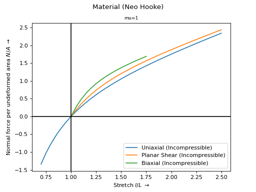
View force-stretch curves on elementary incompressible deformations.

>>> import felupe as fem
>>> import felupe.constitution.tensortrax as mat
>>> import tensortrax.math as tm
>>>
>>> def neo_hooke(C, mu):
...     "Strain energy function of the Neo-Hookean material formulation."
...     return mu / 2 * (tm.linalg.det(C) ** (-1/3) * tm.trace(C) - 3)
>>>
>>> umat = mat.Hyperelastic(neo_hooke, mu=1)
>>> ax = umat.plot(incompressible=True)

参考

felupe.constitution.tensortrax.models.hyperelastic.saint_venant_kirchhoff: Strain energy function of the Saint Venant-Kirchhoff material formulation.
felupe.constitution.tensortrax.models.hyperelastic.neo_hooke: Strain energy function of the Neo-Hookean material formulation.
felupe.constitution.tensortrax.models.hyperelastic.mooney_rivlin: Strain energy function of the Mooney-Rivlin material formulation.
felupe.constitution.tensortrax.models.hyperelastic.yeoh: "Strain energy function of the Yeoh material formulation.
felupe.constitution.tensortrax.models.hyperelastic.third_order_deformation: Strain energy function of the Third-Order-Deformation material formulation.
felupe.constitution.tensortrax.models.hyperelastic.ogden: Strain energy function of the Ogden material formulation.
felupe.constitution.tensortrax.models.hyperelastic.arruda_boyce: Strain energy function of the Arruda-Boyce material formulation.
felupe.constitution.tensortrax.models.hyperelastic.extended_tube: Strain energy function of the Extended-Tube material formulation.
felupe.constitution.tensortrax.models.hyperelastic.van_der_waals: Strain energy function of the Van der Waals material formulation.
felupe.constitution.tensortrax.models.hyperelastic.finite_strain_viscoelastic: Finite strain viscoelastic material formulation.

copy()#: Return a deep-copy of the constitutive material.

gradient(x)#

Return the evaluated gradient of the strain energy density function.

パラメータ:: x (list of ndarray) -- The list with input arguments. These contain the extracted fields of a FieldContainer along with the old vector of state variables, [*field.extract(), statevars_old].
戻り値:: A list with the evaluated gradient(s) of the strain energy density function and the updated vector of state variables.
戻り値の型:: list of ndarray

hessian(x)#

Return the evaluated upper-triangle components of the hessian(s) of the strain energy density function.

パラメータ:: x (list of ndarray) -- The list with input arguments. These contain the extracted fields of a FieldContainer along with the old vector of state variables, [*field.extract(), statevars_old].
戻り値:: A list with the evaluated upper-triangle components of the hessian(s) of the strain energy density function.
戻り値の型:: list of ndarray

is_stable(x, hessian=None)#

Return a boolean mask for stability of isotropic material model formulations.

At a given deformation gradient, a normal force is applied on each principal stretch direction. If the resulting incremental stretches are positive, the material model formulation is considered to be stable at the given deformation gradient.

パラメータ:

x (list of ndarray) -- The list with input arguments. These contain the extracted fields of a FieldContainer.
hessian (ndarray or None, optional) -- Second partial derivative of the strain energy density function w.r.t. the deformation gradient. Default is None.

戻り値:

Boolean mask of stability.

戻り値の型:

ndarray

メモ

警告

This stability check will lead to a singular matrix for isotropic (hyperelastic) material model formulations without a volumetric part.

サンプル

First, let's check the stability of the Neo-Hookean material model formulation. The stability is evaluated on (valid) principal stretches of a biaxial deformation. All deformations are stable.

>>> import numpy as np
>>> import felupe as fem
>>>
>>> umat = fem.NeoHooke(mu=1.0, bulk=2.0)
>>> view = umat.view()
>>> λ = view.biaxial()[0]
>>>
>>> F = np.zeros((3, 3, 1, λ[0].size))
>>> for a in range(3):
...     F[a, a] = λ[a]
>>>
>>> umat.is_stable([F])
array([[ True,  True,  True,  True,  True,  True,  True,  True,  True,
         True,  True,  True,  True,  True,  True,  True]])

Now, let's check the stability of the Mooney-Rivlin material model formulation. The stability is evaluated on (valid) principal stretches of a biaxial deformation. Biaxial deformations are only stable up to a longitudinal stretch of 1.35.

>>> import numpy as np
>>> import felupe as fem
>>> import felupe.constitution.tensortrax as mat
>>>
>>> umat = fem.Hyperelastic(
...     mat.models.hyperelastic.mooney_rivlin,
...     C10=0.25,
...     C01=0.25,
... ) & fem.Volumetric(bulk=5000)
>>> view = umat.view()
>>> λ = view.biaxial()[0]
>>>
>>> F = np.zeros((3, 3, 1, λ[0].size))
>>> for a in range(3):
...     F[a, a] = λ[a]
>>>
>>> umat.is_stable([F])
array([[ True,  True,  True,  True,  True,  True,  True,  True, False,
        False, False, False, False, False, False, False]])

optimize(ux=None, ps=None, bx=None, incompressible=False, relative=False, **kwargs)#

Optimize the material parameters by a least-squares fit on experimental stretch-stress data.

パラメータ:

ux (array of shape (2, ...) or None, optional) -- Experimental uniaxial stretch and force-per-undeformed-area data (default is None).
ps (array of shape (2, ...) or None, optional) -- Experimental planar-shear stretch and force-per-undeformed-area data (default is None).
bx (array of shape (2, ...) or None, optional) -- Experimental biaxial stretch and force-per-undeformed-area data (default is None).
incompressible (bool, optional) -- A flag to enforce incompressible deformations (default is False).
relative (bool, optional) -- A flag to optimize relative instead of absolute residuals, i.e. (predicted - observed) / observed instead of predicted - observed (default is False).
**kwargs (dict, optional) -- Optional keyword arguments are passed to scipy.optimize.least_squares().

戻り値:

ConstitutiveMaterial -- A copy of the constitutive material with the optimized material parameters.
scipy.optimize.OptimizeResult -- Represents the optimization result.

メモ

警告

At least one load case, i.e. one of the arguments ux, ps or bx must not be None.

注釈

For JAX-based materials, double-precision is required to optimize material parameters.

import jax

jax.config.update("jax_enable_x64", True)

The vector of residuals is given in Eq. (3) in case of absolute residuals

(1)#\[ \begin{align}\begin{aligned}\begin{split}\boldsymbol{r} &= \begin{bmatrix} \boldsymbol{r}_\text{ux} \\ \boldsymbol{r}_\text{ps} \\ \boldsymbol{r}_\text{bx} \end{bmatrix}\end{split}\\r_\text{ux}(\lambda_i) &= P_\text{ux}(\lambda_i) - P_\text{ux, observed}(\lambda_i)\\r_\text{ps}(\lambda_i) &= P_\text{ps}(\lambda_i) - P_\text{ps, observed}(\lambda_i)\\r_\text{bx}(\lambda_i) &= P_\text{bx}(\lambda_i) - P_\text{bx, observed}(\lambda_i)\end{aligned}\end{align} \]

and in Eq. (4) in case of relative residuals.

(2)#\[ \begin{align}\begin{aligned}\begin{split}\boldsymbol{r} &= \begin{bmatrix} \boldsymbol{r}_\text{ux} \\ \boldsymbol{r}_\text{ps} \\ \boldsymbol{r}_\text{bx} \end{bmatrix}\end{split}\\r_\text{ux}(\lambda_i) &= \frac{ P_\text{ux}(\lambda_i) - P_\text{ux, observed}(\lambda_i)}{ P_\text{ux, observed}(\lambda_i) }\\r_\text{ps}(\lambda_i) &= \frac{ P_\text{ps}(\lambda_i) - P_\text{ps, observed}(\lambda_i)}{ P_\text{ps, observed}(\lambda_i) }\\r_\text{bx}(\lambda_i) &= \frac{ P_\text{bx}(\lambda_i) - P_\text{bx, observed}(\lambda_i)}{ P_\text{bx, observed}(\lambda_i) }\end{aligned}\end{align} \]

サンプル

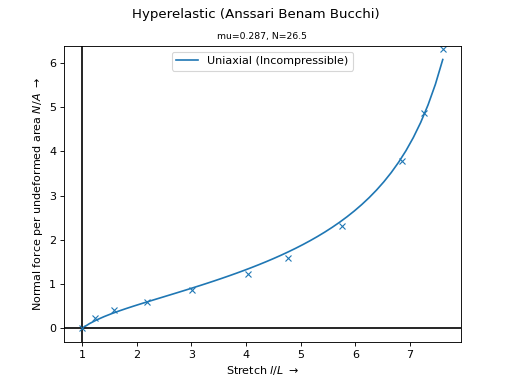
The Anssari-Benam Bucchi material model formulation is best-fitted on Treloar's uniaxial and biaxial tension data [1]_.

>>> import numpy as np
>>> import felupe as fem
>>>
>>> λ, P = np.array(
...     [
...         [1.000, 0.00],
...         [1.240, 2.30],
...         [1.585, 4.16],
...         [2.180, 6.00],
...         [3.020, 8.80],
...         [4.030, 12.5],
...         [4.760, 16.2],
...         [5.750, 23.6],
...         [6.850, 38.5],
...         [7.250, 49.6],
...         [7.600, 64.4],
...     ]
... ).T * np.array([[1.0], [0.0980665]])
>>>
>>> umat = fem.Hyperelastic(fem.anssari_benam_bucchi)
>>> umat_new, res = umat.optimize(
...     ux=[λ, P], incompressible=True, relative=True
... )
>>>
>>> ux = np.linspace(λ.min(), λ.max(), num=50)
>>> ax = umat_new.plot(incompressible=True, ux=ux, bx=None, ps=None)
>>> ax.plot(λ, P, "C0x")

参考

scipy.optimize.least_squares: Solve a nonlinear least-squares problem with bounds on the variables.

参照

plot(incompressible=False, **kwargs)#

Return a plot with normal force per undeformed area vs. stretch curves for the elementary homogeneous deformations uniaxial tension/compression, planar shear and biaxial tension of a given isotropic material formulation.

パラメータ:

incompressible (bool, optional) -- A flag to enforce views on incompressible deformations (default is False).
**kwargs (dict, optional) -- Optional keyword-arguments for ViewMaterial or ViewMaterialIncompressible.

戻り値の型:

matplotlib.axes.Axes

参考

felupe.ViewMaterial: Create views on normal force per undeformed area vs. stretch curves for the elementary homogeneous deformations uniaxial tension/compression, planar shear and biaxial tension of a given isotropic material formulation.
felupe.ViewMaterialIncompressible: Create views on normal force per undeformed area vs. stretch curves for the elementary homogeneous incompressible deformations uniaxial tension/compression, planar shear and biaxial tension of a given isotropic material formulation.

screenshot(filename='umat.png', incompressible=False, **kwargs)#

Save a screenshot with normal force per undeformed area vs. stretch curves for the elementary homogeneous deformations uniaxial tension/compression, planar shear and biaxial tension of a given isotropic material formulation.

パラメータ:

filename (str, optional) -- The filename of the screenshot (default is "umat.png").
incompressible (bool, optional) -- A flag to enforce views on incompressible deformations (default is False).
**kwargs (dict, optional) -- Optional keyword-arguments for ViewMaterial or ViewMaterialIncompressible.

戻り値の型:

matplotlib.axes.Axes

参考

felupe.ViewMaterial: Create views on normal force per undeformed area vs. stretch curves for the elementary homogeneous deformations uniaxial tension/compression, planar shear and biaxial tension of a given isotropic material formulation.
felupe.ViewMaterialIncompressible: Create views on normal force per undeformed area vs. stretch curves for the elementary homogeneous incompressible deformations uniaxial tension/compression, planar shear and biaxial tension of a given isotropic material formulation.

view(incompressible=False, **kwargs)#

Create views on normal force per undeformed area vs. stretch curves for the elementary homogeneous deformations uniaxial tension/compression, planar shear and biaxial tension of a given isotropic material formulation.

パラメータ:

incompressible (bool, optional) -- A flag to enforce views on incompressible deformations (default is False).
**kwargs (dict, optional) -- Optional keyword-arguments for ViewMaterial or ViewMaterialIncompressible.

戻り値の型:

felupe.ViewMaterial or felupe.ViewMaterialIncompressible

参考

felupe.ViewMaterial: Create views on normal force per undeformed area vs. stretch curves for the elementary homogeneous deformations uniaxial tension/compression, planar shear and biaxial tension of a given isotropic material formulation.
felupe.ViewMaterialIncompressible: Create views on normal force per undeformed area vs. stretch curves for the elementary homogeneous incompressible deformations uniaxial tension/compression, planar shear and biaxial tension of a given isotropic material formulation.

class felupe.constitution.tensortrax.Material(fun, nstatevars=0, parallel=False, **kwargs)[ソース]#

A material definition with a given function for the partial derivative of the strain energy function w.r.t. the deformation gradient tensor with Automatic Differentiation provided by tensortrax.

パラメータ:

fun (callable) -- A gradient of the strain energy density function w.r.t. the deformation gradient tensor \(\boldsymbol{F}\). Function signature must be fun = lambda F, **kwargs: P for functions without state variables and fun = lambda F, statevars, **kwargs: [P, statevars_new] for functions with state variables. The deformation gradient tensor will be a tensortrax.Tensor when the function is evaluated. It is important to use only differentiable math-functions from tensortrax.math!
nstatevars (int, optional) -- Number of state variables (default is 0).
parallel (bool, optional) -- A flag to invoke threaded gradient of strain energy density function evaluations (default is False). May introduce additional overhead for small-sized problems.
**kwargs (dict, optional) -- Optional keyword-arguments for the gradient of the strain energy density function.

メモ

The gradient of the strain energy density function \(\frac{\partial \psi}{\partial \boldsymbol{F}}\) must be given in terms of the deformation gradient tensor \(\boldsymbol{F}\).

警告

It is important to use only differentiable math-functions from tensortrax.math!

\[\boldsymbol{P} = \frac{\partial \psi(\boldsymbol{F}, \boldsymbol{\zeta})}{ \partial \boldsymbol{F}}\]

Take this code-block as template

import felupe as fem
import felupe.constitution.tensortrax as mat
import tensortrax.math as tm

def neo_hooke(F, mu):
    "First Piola-Kirchhoff stress of the Neo-Hookean material formulation."

    C = tm.dot(tm.transpose(F), F)
    Cu = tm.linalg.det(C) ** (-1/3) * C

    return mu * F @ tm.special.dev(Cu) @ tm.linalg.inv(C)

umat = mat.Material(neo_hooke, mu=1)

and this code-block for material formulations with state variables:

import felupe as fem
import felupe.constitution.tensortrax as mat
import tensortrax.math as tm

def viscoelastic(F, Cin, mu, eta, dtime):
    "Finite strain viscoelastic material formulation."

    # unimodular part of the right Cauchy-Green deformation tensor
    C = tm.dot(tm.transpose(F), F)
    Cu = tm.linalg.det(C) ** (-1 / 3) * C

    # update of state variables by evolution equation
    Ci = tm.special.from_triu_1d(Cin, like=C) + mu / eta * dtime * Cu
    Ci = tm.linalg.det(Ci) ** (-1 / 3) * Ci

    # second Piola-Kirchhoff stress tensor
    S = mu * tm.special.dev(Cu @ tm.linalg.inv(Ci)) @ tm.linalg.inv(C)

    # first Piola-Kirchhoff stress tensor and state variable
    return F @ S, tm.special.triu_1d(Ci)

umat = mat.Material(viscoelastic, mu=1, eta=1, dtime=1, nstatevars=6)

注釈

See the documentation of tensortrax for further details.

サンプル

>>> import felupe as fem
>>> import felupe.constitution.tensortrax as mat
>>> import tensortrax.math as tm
>>>
>>> def neo_hooke(F, mu):
...     C = tm.dot(tm.transpose(F), F)
...     S = mu * tm.special.dev(tm.linalg.det(C)**(-1/3) * C) @ tm.linalg.inv(C)
...     return F @ S
>>>
>>> umat = mat.Material(neo_hooke, mu=1)
>>> ax = umat.plot(incompressible=True)

copy()#: Return a deep-copy of the constitutive material.

gradient(x)[ソース]#

Return the evaluated gradient of the strain energy density function.

パラメータ:: x (list of ndarray) -- The list with input arguments. These contain the extracted fields of a FieldContainer along with the old vector of state variables, [*field.extract(), statevars_old].
戻り値:: A list with the evaluated gradient(s) of the strain energy density function and the updated vector of state variables.
戻り値の型:: list of ndarray

hessian(x)[ソース]#

Return the evaluated upper-triangle components of the hessian(s) of the strain energy density function.

パラメータ:: x (list of ndarray) -- The list with input arguments. These contain the extracted fields of a FieldContainer along with the old vector of state variables, [*field.extract(), statevars_old].
戻り値:: A list with the evaluated upper-triangle components of the hessian(s) of the strain energy density function.
戻り値の型:: list of ndarray

is_stable(x, hessian=None)#

Return a boolean mask for stability of isotropic material model formulations.

At a given deformation gradient, a normal force is applied on each principal stretch direction. If the resulting incremental stretches are positive, the material model formulation is considered to be stable at the given deformation gradient.

パラメータ:

x (list of ndarray) -- The list with input arguments. These contain the extracted fields of a FieldContainer.
hessian (ndarray or None, optional) -- Second partial derivative of the strain energy density function w.r.t. the deformation gradient. Default is None.

戻り値:

Boolean mask of stability.

戻り値の型:

ndarray

メモ

警告

This stability check will lead to a singular matrix for isotropic (hyperelastic) material model formulations without a volumetric part.

サンプル

First, let's check the stability of the Neo-Hookean material model formulation. The stability is evaluated on (valid) principal stretches of a biaxial deformation. All deformations are stable.

>>> import numpy as np
>>> import felupe as fem
>>>
>>> umat = fem.NeoHooke(mu=1.0, bulk=2.0)
>>> view = umat.view()
>>> λ = view.biaxial()[0]
>>>
>>> F = np.zeros((3, 3, 1, λ[0].size))
>>> for a in range(3):
...     F[a, a] = λ[a]
>>>
>>> umat.is_stable([F])
array([[ True,  True,  True,  True,  True,  True,  True,  True,  True,
         True,  True,  True,  True,  True,  True,  True]])

Now, let's check the stability of the Mooney-Rivlin material model formulation. The stability is evaluated on (valid) principal stretches of a biaxial deformation. Biaxial deformations are only stable up to a longitudinal stretch of 1.35.

>>> import numpy as np
>>> import felupe as fem
>>> import felupe.constitution.tensortrax as mat
>>>
>>> umat = fem.Hyperelastic(
...     mat.models.hyperelastic.mooney_rivlin,
...     C10=0.25,
...     C01=0.25,
... ) & fem.Volumetric(bulk=5000)
>>> view = umat.view()
>>> λ = view.biaxial()[0]
>>>
>>> F = np.zeros((3, 3, 1, λ[0].size))
>>> for a in range(3):
...     F[a, a] = λ[a]
>>>
>>> umat.is_stable([F])
array([[ True,  True,  True,  True,  True,  True,  True,  True, False,
        False, False, False, False, False, False, False]])

optimize(ux=None, ps=None, bx=None, incompressible=False, relative=False, **kwargs)#

Optimize the material parameters by a least-squares fit on experimental stretch-stress data.

パラメータ:

ux (array of shape (2, ...) or None, optional) -- Experimental uniaxial stretch and force-per-undeformed-area data (default is None).
ps (array of shape (2, ...) or None, optional) -- Experimental planar-shear stretch and force-per-undeformed-area data (default is None).
bx (array of shape (2, ...) or None, optional) -- Experimental biaxial stretch and force-per-undeformed-area data (default is None).
incompressible (bool, optional) -- A flag to enforce incompressible deformations (default is False).
relative (bool, optional) -- A flag to optimize relative instead of absolute residuals, i.e. (predicted - observed) / observed instead of predicted - observed (default is False).
**kwargs (dict, optional) -- Optional keyword arguments are passed to scipy.optimize.least_squares().

戻り値:

ConstitutiveMaterial -- A copy of the constitutive material with the optimized material parameters.
scipy.optimize.OptimizeResult -- Represents the optimization result.

メモ

警告

At least one load case, i.e. one of the arguments ux, ps or bx must not be None.

注釈

For JAX-based materials, double-precision is required to optimize material parameters.

import jax

jax.config.update("jax_enable_x64", True)

The vector of residuals is given in Eq. (3) in case of absolute residuals

(3)#\[ \begin{align}\begin{aligned}\begin{split}\boldsymbol{r} &= \begin{bmatrix} \boldsymbol{r}_\text{ux} \\ \boldsymbol{r}_\text{ps} \\ \boldsymbol{r}_\text{bx} \end{bmatrix}\end{split}\\r_\text{ux}(\lambda_i) &= P_\text{ux}(\lambda_i) - P_\text{ux, observed}(\lambda_i)\\r_\text{ps}(\lambda_i) &= P_\text{ps}(\lambda_i) - P_\text{ps, observed}(\lambda_i)\\r_\text{bx}(\lambda_i) &= P_\text{bx}(\lambda_i) - P_\text{bx, observed}(\lambda_i)\end{aligned}\end{align} \]

and in Eq. (4) in case of relative residuals.

(4)#\[ \begin{align}\begin{aligned}\begin{split}\boldsymbol{r} &= \begin{bmatrix} \boldsymbol{r}_\text{ux} \\ \boldsymbol{r}_\text{ps} \\ \boldsymbol{r}_\text{bx} \end{bmatrix}\end{split}\\r_\text{ux}(\lambda_i) &= \frac{ P_\text{ux}(\lambda_i) - P_\text{ux, observed}(\lambda_i)}{ P_\text{ux, observed}(\lambda_i) }\\r_\text{ps}(\lambda_i) &= \frac{ P_\text{ps}(\lambda_i) - P_\text{ps, observed}(\lambda_i)}{ P_\text{ps, observed}(\lambda_i) }\\r_\text{bx}(\lambda_i) &= \frac{ P_\text{bx}(\lambda_i) - P_\text{bx, observed}(\lambda_i)}{ P_\text{bx, observed}(\lambda_i) }\end{aligned}\end{align} \]

サンプル

The Anssari-Benam Bucchi material model formulation is best-fitted on Treloar's uniaxial and biaxial tension data [1]_.

>>> import numpy as np
>>> import felupe as fem
>>>
>>> λ, P = np.array(
...     [
...         [1.000, 0.00],
...         [1.240, 2.30],
...         [1.585, 4.16],
...         [2.180, 6.00],
...         [3.020, 8.80],
...         [4.030, 12.5],
...         [4.760, 16.2],
...         [5.750, 23.6],
...         [6.850, 38.5],
...         [7.250, 49.6],
...         [7.600, 64.4],
...     ]
... ).T * np.array([[1.0], [0.0980665]])
>>>
>>> umat = fem.Hyperelastic(fem.anssari_benam_bucchi)
>>> umat_new, res = umat.optimize(
...     ux=[λ, P], incompressible=True, relative=True
... )
>>>
>>> ux = np.linspace(λ.min(), λ.max(), num=50)
>>> ax = umat_new.plot(incompressible=True, ux=ux, bx=None, ps=None)
>>> ax.plot(λ, P, "C0x")

参考

scipy.optimize.least_squares: Solve a nonlinear least-squares problem with bounds on the variables.

参照

plot(incompressible=False, **kwargs)#

Return a plot with normal force per undeformed area vs. stretch curves for the elementary homogeneous deformations uniaxial tension/compression, planar shear and biaxial tension of a given isotropic material formulation.

パラメータ:

incompressible (bool, optional) -- A flag to enforce views on incompressible deformations (default is False).
**kwargs (dict, optional) -- Optional keyword-arguments for ViewMaterial or ViewMaterialIncompressible.

戻り値の型:

matplotlib.axes.Axes

参考

felupe.ViewMaterial: Create views on normal force per undeformed area vs. stretch curves for the elementary homogeneous deformations uniaxial tension/compression, planar shear and biaxial tension of a given isotropic material formulation.
felupe.ViewMaterialIncompressible: Create views on normal force per undeformed area vs. stretch curves for the elementary homogeneous incompressible deformations uniaxial tension/compression, planar shear and biaxial tension of a given isotropic material formulation.

screenshot(filename='umat.png', incompressible=False, **kwargs)#

Save a screenshot with normal force per undeformed area vs. stretch curves for the elementary homogeneous deformations uniaxial tension/compression, planar shear and biaxial tension of a given isotropic material formulation.

パラメータ:

filename (str, optional) -- The filename of the screenshot (default is "umat.png").
incompressible (bool, optional) -- A flag to enforce views on incompressible deformations (default is False).
**kwargs (dict, optional) -- Optional keyword-arguments for ViewMaterial or ViewMaterialIncompressible.

戻り値の型:

matplotlib.axes.Axes

参考

felupe.ViewMaterial: Create views on normal force per undeformed area vs. stretch curves for the elementary homogeneous deformations uniaxial tension/compression, planar shear and biaxial tension of a given isotropic material formulation.
felupe.ViewMaterialIncompressible: Create views on normal force per undeformed area vs. stretch curves for the elementary homogeneous incompressible deformations uniaxial tension/compression, planar shear and biaxial tension of a given isotropic material formulation.

view(incompressible=False, **kwargs)#

Create views on normal force per undeformed area vs. stretch curves for the elementary homogeneous deformations uniaxial tension/compression, planar shear and biaxial tension of a given isotropic material formulation.

パラメータ:

incompressible (bool, optional) -- A flag to enforce views on incompressible deformations (default is False).
**kwargs (dict, optional) -- Optional keyword-arguments for ViewMaterial or ViewMaterialIncompressible.

戻り値の型:

felupe.ViewMaterial or felupe.ViewMaterialIncompressible

参考

felupe.ViewMaterial: Create views on normal force per undeformed area vs. stretch curves for the elementary homogeneous deformations uniaxial tension/compression, planar shear and biaxial tension of a given isotropic material formulation.
felupe.ViewMaterialIncompressible: Create views on normal force per undeformed area vs. stretch curves for the elementary homogeneous incompressible deformations uniaxial tension/compression, planar shear and biaxial tension of a given isotropic material formulation.

class felupe.Hyperelastic(fun, nstatevars=0, parallel=False, **kwargs)[ソース]#

A hyperelastic material definition with a given function for the strain energy density function per unit undeformed volume with Automatic Differentiation provided by tensortrax.

パラメータ:

fun (callable) -- A strain energy density function in terms of the right Cauchy-Green deformation tensor \(\boldsymbol{C}\). Function signature must be fun = lambda C, **kwargs: psi for functions without state variables and fun = lambda C, statevars, **kwargs: [psi, statevars_new] for functions with state variables. The right Cauchy-Green deformation tensor will be a tensortrax.Tensor when the function is evaluated. It is important to use only differentiable math-functions from tensortrax.math.
nstatevars (int, optional) -- Number of state variables (default is 0).
parallel (bool, optional) -- A flag to invoke threaded strain energy density function evaluations (default is False). May introduce additional overhead for small-sized problems.
**kwargs (dict, optional) -- Optional keyword-arguments for the strain energy density function.

メモ

The strain energy density function \(\psi\) must be given in terms of the right Cauchy-Green deformation tensor \(\boldsymbol{C} = \boldsymbol{F}^T \boldsymbol{F}\).

警告

It is important to use only differentiable math-functions from tensortrax.math!

Take this minimal code-block as template

\[\psi = \psi(\boldsymbol{C})\]

import felupe as fem
import felupe.constitution.tensortrax as mat
import tensortrax.math as tm

def neo_hooke(C, mu):
    "Strain energy function of the Neo-Hookean material formulation."
    return mu / 2 * (tm.linalg.det(C) ** (-1/3) * tm.trace(C) - 3)

umat = mat.Hyperelastic(neo_hooke, mu=1)

and this code-block for material formulations with state variables.

\[\psi = \psi(\boldsymbol{C}, \boldsymbol{\zeta})\]

import felupe as fem
import felupe.constitution.tensortrax as mat
import tensortrax.math as tm

def viscoelastic(C, Cin, mu, eta, dtime):
    "Finite strain viscoelastic material formulation."

    # unimodular part of the right Cauchy-Green deformation tensor
    Cu = tm.linalg.det(C) ** (-1 / 3) * C

    # update of state variables by evolution equation
    Ci = tm.special.from_triu_1d(Cin, like=C) + mu / eta * dtime * Cu
    Ci = tm.linalg.det(Ci) ** (-1 / 3) * Ci

    # first invariant of elastic part of right Cauchy-Green deformation tensor
    I1 = tm.trace(Cu @ tm.linalg.inv(Ci))

    # strain energy function and state variable
    return mu / 2 * (I1 - 3), tm.special.triu_1d(Ci)

umat = mat.Hyperelastic(viscoelastic, mu=1, eta=1, dtime=1, nstatevars=6)

注釈

See the documentation of tensortrax for further details.

サンプル

View force-stretch curves on elementary incompressible deformations.

>>> import felupe as fem
>>> import felupe.constitution.tensortrax as mat
>>> import tensortrax.math as tm
>>>
>>> def neo_hooke(C, mu):
...     "Strain energy function of the Neo-Hookean material formulation."
...     return mu / 2 * (tm.linalg.det(C) ** (-1/3) * tm.trace(C) - 3)
>>>
>>> umat = mat.Hyperelastic(neo_hooke, mu=1)
>>> ax = umat.plot(incompressible=True)

参考

felupe.constitution.tensortrax.models.hyperelastic.saint_venant_kirchhoff: Strain energy function of the Saint Venant-Kirchhoff material formulation.
felupe.constitution.tensortrax.models.hyperelastic.neo_hooke: Strain energy function of the Neo-Hookean material formulation.
felupe.constitution.tensortrax.models.hyperelastic.mooney_rivlin: Strain energy function of the Mooney-Rivlin material formulation.
felupe.constitution.tensortrax.models.hyperelastic.yeoh: "Strain energy function of the Yeoh material formulation.
felupe.constitution.tensortrax.models.hyperelastic.third_order_deformation: Strain energy function of the Third-Order-Deformation material formulation.
felupe.constitution.tensortrax.models.hyperelastic.ogden: Strain energy function of the Ogden material formulation.
felupe.constitution.tensortrax.models.hyperelastic.arruda_boyce: Strain energy function of the Arruda-Boyce material formulation.
felupe.constitution.tensortrax.models.hyperelastic.extended_tube: Strain energy function of the Extended-Tube material formulation.
felupe.constitution.tensortrax.models.hyperelastic.van_der_waals: Strain energy function of the Van der Waals material formulation.
felupe.constitution.tensortrax.models.hyperelastic.finite_strain_viscoelastic: Finite strain viscoelastic material formulation.

copy()#: Return a deep-copy of the constitutive material.

gradient(x)#

Return the evaluated gradient of the strain energy density function.

パラメータ:: x (list of ndarray) -- The list with input arguments. These contain the extracted fields of a FieldContainer along with the old vector of state variables, [*field.extract(), statevars_old].
戻り値:: A list with the evaluated gradient(s) of the strain energy density function and the updated vector of state variables.
戻り値の型:: list of ndarray

hessian(x)#

Return the evaluated upper-triangle components of the hessian(s) of the strain energy density function.

パラメータ:: x (list of ndarray) -- The list with input arguments. These contain the extracted fields of a FieldContainer along with the old vector of state variables, [*field.extract(), statevars_old].
戻り値:: A list with the evaluated upper-triangle components of the hessian(s) of the strain energy density function.
戻り値の型:: list of ndarray

is_stable(x, hessian=None)#

Return a boolean mask for stability of isotropic material model formulations.

At a given deformation gradient, a normal force is applied on each principal stretch direction. If the resulting incremental stretches are positive, the material model formulation is considered to be stable at the given deformation gradient.

パラメータ:

x (list of ndarray) -- The list with input arguments. These contain the extracted fields of a FieldContainer.
hessian (ndarray or None, optional) -- Second partial derivative of the strain energy density function w.r.t. the deformation gradient. Default is None.

戻り値:

Boolean mask of stability.

戻り値の型:

ndarray

メモ

警告

This stability check will lead to a singular matrix for isotropic (hyperelastic) material model formulations without a volumetric part.

サンプル

First, let's check the stability of the Neo-Hookean material model formulation. The stability is evaluated on (valid) principal stretches of a biaxial deformation. All deformations are stable.

>>> import numpy as np
>>> import felupe as fem
>>>
>>> umat = fem.NeoHooke(mu=1.0, bulk=2.0)
>>> view = umat.view()
>>> λ = view.biaxial()[0]
>>>
>>> F = np.zeros((3, 3, 1, λ[0].size))
>>> for a in range(3):
...     F[a, a] = λ[a]
>>>
>>> umat.is_stable([F])
array([[ True,  True,  True,  True,  True,  True,  True,  True,  True,
         True,  True,  True,  True,  True,  True,  True]])

Now, let's check the stability of the Mooney-Rivlin material model formulation. The stability is evaluated on (valid) principal stretches of a biaxial deformation. Biaxial deformations are only stable up to a longitudinal stretch of 1.35.

>>> import numpy as np
>>> import felupe as fem
>>> import felupe.constitution.tensortrax as mat
>>>
>>> umat = fem.Hyperelastic(
...     mat.models.hyperelastic.mooney_rivlin,
...     C10=0.25,
...     C01=0.25,
... ) & fem.Volumetric(bulk=5000)
>>> view = umat.view()
>>> λ = view.biaxial()[0]
>>>
>>> F = np.zeros((3, 3, 1, λ[0].size))
>>> for a in range(3):
...     F[a, a] = λ[a]
>>>
>>> umat.is_stable([F])
array([[ True,  True,  True,  True,  True,  True,  True,  True, False,
        False, False, False, False, False, False, False]])

optimize(ux=None, ps=None, bx=None, incompressible=False, relative=False, **kwargs)#

Optimize the material parameters by a least-squares fit on experimental stretch-stress data.

パラメータ:

ux (array of shape (2, ...) or None, optional) -- Experimental uniaxial stretch and force-per-undeformed-area data (default is None).
ps (array of shape (2, ...) or None, optional) -- Experimental planar-shear stretch and force-per-undeformed-area data (default is None).
bx (array of shape (2, ...) or None, optional) -- Experimental biaxial stretch and force-per-undeformed-area data (default is None).
incompressible (bool, optional) -- A flag to enforce incompressible deformations (default is False).
relative (bool, optional) -- A flag to optimize relative instead of absolute residuals, i.e. (predicted - observed) / observed instead of predicted - observed (default is False).
**kwargs (dict, optional) -- Optional keyword arguments are passed to scipy.optimize.least_squares().

戻り値:

ConstitutiveMaterial -- A copy of the constitutive material with the optimized material parameters.
scipy.optimize.OptimizeResult -- Represents the optimization result.

メモ

警告

At least one load case, i.e. one of the arguments ux, ps or bx must not be None.

注釈

For JAX-based materials, double-precision is required to optimize material parameters.

import jax

jax.config.update("jax_enable_x64", True)

The vector of residuals is given in Eq. (3) in case of absolute residuals

(5)#\[ \begin{align}\begin{aligned}\begin{split}\boldsymbol{r} &= \begin{bmatrix} \boldsymbol{r}_\text{ux} \\ \boldsymbol{r}_\text{ps} \\ \boldsymbol{r}_\text{bx} \end{bmatrix}\end{split}\\r_\text{ux}(\lambda_i) &= P_\text{ux}(\lambda_i) - P_\text{ux, observed}(\lambda_i)\\r_\text{ps}(\lambda_i) &= P_\text{ps}(\lambda_i) - P_\text{ps, observed}(\lambda_i)\\r_\text{bx}(\lambda_i) &= P_\text{bx}(\lambda_i) - P_\text{bx, observed}(\lambda_i)\end{aligned}\end{align} \]

and in Eq. (4) in case of relative residuals.

(6)#\[ \begin{align}\begin{aligned}\begin{split}\boldsymbol{r} &= \begin{bmatrix} \boldsymbol{r}_\text{ux} \\ \boldsymbol{r}_\text{ps} \\ \boldsymbol{r}_\text{bx} \end{bmatrix}\end{split}\\r_\text{ux}(\lambda_i) &= \frac{ P_\text{ux}(\lambda_i) - P_\text{ux, observed}(\lambda_i)}{ P_\text{ux, observed}(\lambda_i) }\\r_\text{ps}(\lambda_i) &= \frac{ P_\text{ps}(\lambda_i) - P_\text{ps, observed}(\lambda_i)}{ P_\text{ps, observed}(\lambda_i) }\\r_\text{bx}(\lambda_i) &= \frac{ P_\text{bx}(\lambda_i) - P_\text{bx, observed}(\lambda_i)}{ P_\text{bx, observed}(\lambda_i) }\end{aligned}\end{align} \]

サンプル

The Anssari-Benam Bucchi material model formulation is best-fitted on Treloar's uniaxial and biaxial tension data [1]_.

>>> import numpy as np
>>> import felupe as fem
>>>
>>> λ, P = np.array(
...     [
...         [1.000, 0.00],
...         [1.240, 2.30],
...         [1.585, 4.16],
...         [2.180, 6.00],
...         [3.020, 8.80],
...         [4.030, 12.5],
...         [4.760, 16.2],
...         [5.750, 23.6],
...         [6.850, 38.5],
...         [7.250, 49.6],
...         [7.600, 64.4],
...     ]
... ).T * np.array([[1.0], [0.0980665]])
>>>
>>> umat = fem.Hyperelastic(fem.anssari_benam_bucchi)
>>> umat_new, res = umat.optimize(
...     ux=[λ, P], incompressible=True, relative=True
... )
>>>
>>> ux = np.linspace(λ.min(), λ.max(), num=50)
>>> ax = umat_new.plot(incompressible=True, ux=ux, bx=None, ps=None)
>>> ax.plot(λ, P, "C0x")

参考

scipy.optimize.least_squares: Solve a nonlinear least-squares problem with bounds on the variables.

参照

plot(incompressible=False, **kwargs)#

Return a plot with normal force per undeformed area vs. stretch curves for the elementary homogeneous deformations uniaxial tension/compression, planar shear and biaxial tension of a given isotropic material formulation.

パラメータ:

incompressible (bool, optional) -- A flag to enforce views on incompressible deformations (default is False).
**kwargs (dict, optional) -- Optional keyword-arguments for ViewMaterial or ViewMaterialIncompressible.

戻り値の型:

matplotlib.axes.Axes

参考

felupe.ViewMaterial: Create views on normal force per undeformed area vs. stretch curves for the elementary homogeneous deformations uniaxial tension/compression, planar shear and biaxial tension of a given isotropic material formulation.
felupe.ViewMaterialIncompressible: Create views on normal force per undeformed area vs. stretch curves for the elementary homogeneous incompressible deformations uniaxial tension/compression, planar shear and biaxial tension of a given isotropic material formulation.

screenshot(filename='umat.png', incompressible=False, **kwargs)#

Save a screenshot with normal force per undeformed area vs. stretch curves for the elementary homogeneous deformations uniaxial tension/compression, planar shear and biaxial tension of a given isotropic material formulation.

パラメータ:

filename (str, optional) -- The filename of the screenshot (default is "umat.png").
incompressible (bool, optional) -- A flag to enforce views on incompressible deformations (default is False).
**kwargs (dict, optional) -- Optional keyword-arguments for ViewMaterial or ViewMaterialIncompressible.

戻り値の型:

matplotlib.axes.Axes

参考

felupe.ViewMaterial: Create views on normal force per undeformed area vs. stretch curves for the elementary homogeneous deformations uniaxial tension/compression, planar shear and biaxial tension of a given isotropic material formulation.
felupe.ViewMaterialIncompressible: Create views on normal force per undeformed area vs. stretch curves for the elementary homogeneous incompressible deformations uniaxial tension/compression, planar shear and biaxial tension of a given isotropic material formulation.

view(incompressible=False, **kwargs)#

Create views on normal force per undeformed area vs. stretch curves for the elementary homogeneous deformations uniaxial tension/compression, planar shear and biaxial tension of a given isotropic material formulation.

パラメータ:

incompressible (bool, optional) -- A flag to enforce views on incompressible deformations (default is False).
**kwargs (dict, optional) -- Optional keyword-arguments for ViewMaterial or ViewMaterialIncompressible.

戻り値の型:

felupe.ViewMaterial or felupe.ViewMaterialIncompressible

参考

felupe.ViewMaterial: Create views on normal force per undeformed area vs. stretch curves for the elementary homogeneous deformations uniaxial tension/compression, planar shear and biaxial tension of a given isotropic material formulation.
felupe.ViewMaterialIncompressible: Create views on normal force per undeformed area vs. stretch curves for the elementary homogeneous incompressible deformations uniaxial tension/compression, planar shear and biaxial tension of a given isotropic material formulation.

felupe.MaterialAD#: :py:class:`~felupe.constitution.tensortrax._material.Material`の別名です。

felupe.constitution.tensortrax.total_lagrange(material)[ソース]#

Decorate a second Piola-Kirchhoff stress Total-Lagrange material formulation as a first Piola-Kirchoff stress function.

メモ

The Green-Lagrange strain tensor and its first variation are given in Eq. (7).

(7)#\[ \begin{align}\begin{aligned}\boldsymbol{E} &= \frac{1}{2} \left( \boldsymbol{F}^T \boldsymbol{F} - \boldsymbol{1} \right)\\\delta \boldsymbol{E} &= \frac{1}{2} \left( \delta \boldsymbol{F}^T \boldsymbol{F} + \boldsymbol{F}^T \delta \boldsymbol{F} \right)\end{aligned}\end{align} \]

This will lead to the variations of the strain energy density function per unit undeformed volume, see Eq. (8).

(8)#\[ \begin{align}\begin{aligned}\delta \psi &= \boldsymbol{S} : \delta \boldsymbol{E}\\\delta \psi &= \boldsymbol{F} \boldsymbol{S} : \delta \boldsymbol{F}\end{aligned}\end{align} \]

Finally, the first Piola-Kirchhoff stress tensor is given by Eq. (14).

(9)#\[\boldsymbol{P} = \boldsymbol{F} \boldsymbol{S}\]

サンプル

>>> import felupe as fem
>>> import felupe.constitution.tensortrax as mat
>>> import tensortrax.math as tm
>>>
>>> @fem.total_lagrange
... def neo_hooke_total_lagrange(F, mu=1):
...     C = F.T @ F
...     S = mu * tm.special.dev(tm.linalg.det(C)**(-1/3) * C) @ tm.linalg.inv(C)
...     return S
>>>
>>> umat = mat.Material(neo_hooke_total_lagrange, mu=1)

参考

felupe.constitution.tensortrax.Hyperelastic: A hyperelastic material definition with a given function for the strain energy density function per unit undeformed volume with Automatic Differentiation.
felupe.constitution.tensortrax.Material: A material definition with a given function for the partial derivative of the strain energy function w.r.t. the deformation gradient tensor with Automatic Differentiation.

felupe.constitution.tensortrax.updated_lagrange(material)[ソース]#

Decorate a Cauchy-stress Updated-Lagrange material formulation as a first Piola- Kirchoff stress function.

メモ

The equilibrium equations for statics are given in Eq. (10).

(10)#\[\operatorname{div} \boldsymbol{\sigma} + \boldsymbol{b} = \boldsymbol{0}\]

The weak form of the equilibrium equations for statics is given in Eq. (11).

(11)#\[ \begin{align}\begin{aligned}\int_v \operatorname{div} \boldsymbol{\sigma} \cdot \delta \boldsymbol{u} \ \mathrm{d}v + \int_v \boldsymbol{b} \cdot \delta \boldsymbol{u} \ \mathrm{d}v &= 0\\- \int_v \boldsymbol{\sigma} : \frac{\partial \delta \boldsymbol{u}}{\partial \boldsymbol{x}} \ \mathrm{d}v + \int_{\partial v} \left( \boldsymbol{\sigma} \cdot \boldsymbol{n} \right ) \cdot \delta \boldsymbol{u} \ \mathrm{d}a + \int_v \boldsymbol{b} \cdot \delta \boldsymbol{u} \ \mathrm{d}v &= 0\end{aligned}\end{align} \]

This leads to the virtual work of internal forces, see Eq. (12).

(12)#\[\delta W_{\text{int}} = -\int_v \boldsymbol{\sigma} : \frac{\partial \delta \boldsymbol{u}}{\partial \boldsymbol{x}} \ \mathrm{d}v\]

The variation of the total potential energy of internal forces is given in Eq. (13).

(13)#\[ \begin{align}\begin{aligned}\delta \Pi &= \int_v \boldsymbol{\sigma} : \frac{\partial \delta \boldsymbol{u}}{\partial \boldsymbol{x}} \ \mathrm{d}v\\\delta \Pi &= \int_V \boldsymbol{\sigma} : \delta \boldsymbol{F} \boldsymbol{F}^{-1} \ J \mathrm{d}V\\\delta \Pi &= \int_V \boldsymbol{P} : \delta \boldsymbol{F} \ \mathrm{d}V\end{aligned}\end{align} \]

Finally, the first Piola-Kirchhoff stress tensor is given by Eq. (14).

(14)#\[\boldsymbol{P} = J \boldsymbol{\sigma} \boldsymbol{F}^{-T}\]

サンプル

>>> import felupe as fem
>>> import felupe.constitution.tensortrax as mat
>>> import tensortrax.math as tm
>>>
>>> @fem.updated_lagrange
... def neo_hooke_updated_lagrange(F, mu=1):
...     J = tm.linalg.det(F)
...     b = F @ F.T
...     σ = mu * tm.special.dev(J**(-2/3) * b) / J
...     return σ
>>>
>>> umat = mat.Material(neo_hooke_updated_lagrange, mu=1)

参考

felupe.constitution.tensortrax.Hyperelastic: A hyperelastic material definition with a given function for the strain energy density function per unit undeformed volume with Automatic Differentiation.
felupe.constitution.tensortrax.Material: A material definition with a given function for the partial derivative of the strain energy function w.r.t. the deformation gradient tensor with Automatic Differentiation.

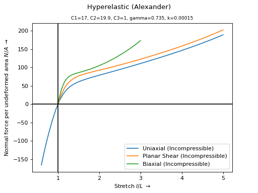
felupe.constitution.tensortrax.models.hyperelastic.alexander(C, C1, C2, C3, gamma, k)[ソース]#

Strain energy function of the isotropic hyperelastic Alexander material formulation [1]_.

パラメータ:

C (tensortrax.Tensor) -- Right Cauchy-Green deformation tensor.
C1 (float) -- Scale factor for the first invariant term.
C2 (float) -- Scale factor for the second invariant term.
C3 (float) -- Scale factor for the logarithmic second invariant term.
gamma (float) -- Offset-normalization parameter for the logarithmic second invariant term.
k (float) -- Scale factor for the exponential first invariant term.

メモ

警告

The strain energy function of the Alexander model formulation is not directly implemented. Only its gradient and hessian w.r.t. the right Cauchy-Green deformation tensor are defined. This is because the imaginary error-function \(\text{erfi}(x)\) is not included in NumPy - this would require SciPy as a dependency.

The strain energy function is given in Eq. (15)

(15)#\[\psi = C_1 \int_{\hat{I}_1} \exp \left( k \left(\hat{I}_1 - 3 \right)^2 \right) \ d\hat{I}_1 + C_2 \ln \left(\frac{\hat{I}_2 - 3 + \gamma}{\gamma} \right) + C_3 \left(\hat{I}_2 - 3 \right)\]

with the first and second main invariant of the distortional part of the right Cauchy-Green deformation tensor, see Eq. (16).

(16)#\[ \begin{align}\begin{aligned}\hat{I}_1 &= J^{-2/3} \text{tr}\left( \boldsymbol{C} \right)\\\hat{I}_2 &= J^{-4/3} \frac{1}{2} \left( \text{tr}\left(\boldsymbol{C}\right)^2 - \text{tr}\left(\boldsymbol{C}^2\right) \right)\end{aligned}\end{align} \]

The initial shear modulus \(\mu\) is given in Eq. (17).

(17)#\[\mu = 2 \left( C_1 + \frac{C_2}{\gamma} + C_3 \right)\]

サンプル

>>> import felupe as fem
>>>
>>> umat = fem.Hyperelastic(
...    fem.alexander, C1=17, C2=19.85, C3=1, gamma=0.735, k=0.00015
... )
>>> ux = fem.math.linsteps([0.6, 5], num=50)
>>> ps = fem.math.linsteps([1, 5], num=50)
>>> bx = fem.math.linsteps([1, 3], num=50)
>>>
>>> ax = umat.plot(ux=ux, ps=ps, bx=bx, incompressible=True)

参照

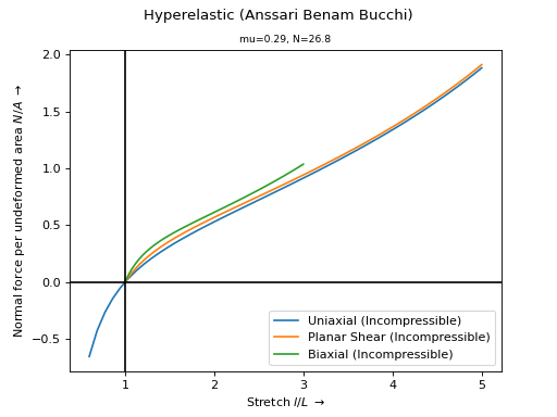
felupe.constitution.tensortrax.models.hyperelastic.anssari_benam_bucchi(C, mu, N)[ソース]#

Strain energy function of the isotropic hyperelastic generalized Neo-Hookean Anssari-Benam Bucchi material formulation [1]_.

パラメータ:

C (tensortrax.Tensor) -- Right Cauchy-Green deformation tensor.
mu (float) -- Modulus \(\mu = nkT\) - this is not the infinitesimal shear modulus.
N (float) -- Number of Kuhn segments of a chain.

メモ

The strain energy function is given in Eq. (18)

(18)#\[\psi = \mu N \left( \frac{1}{6N} \left( \hat{I}_1 - 3 \right) - \ln \left( \frac{\hat{I}_1 - 3N}{3 - 3N} \right) \right)\]

with the first main invariant of the distortional part of the right Cauchy-Green deformation tensor, see Eq. (19).

(19)#\[\hat{I}_1 = J^{-2/3} \text{tr}\left( \boldsymbol{C} \right)\]

The initial shear modulus \(\mu_0\) is given in Eq. (20).

(20)#\[\mu_0 = \mu \frac{1 - 3N}{3 - 3N}\]

サンプル

>>> import felupe as fem
>>>
>>> umat = fem.Hyperelastic(fem.anssari_benam_bucchi, mu=0.29, N=26.8)
>>>
>>> ux = fem.math.linsteps([0.6, 5], num=50)
>>> ps = fem.math.linsteps([1, 5], num=50)
>>> bx = fem.math.linsteps([1, 3], num=50)
>>>
>>> ax = umat.plot(ux=ux, ps=ps, bx=bx, incompressible=True)

参照

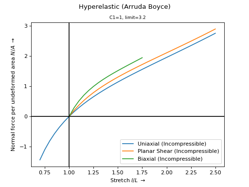
felupe.constitution.tensortrax.models.hyperelastic.arruda_boyce(C, C1, limit)[ソース]#

Strain energy function of the isotropic hyperelastic Arruda-Boyce material formulation.

パラメータ:

C (tensortrax.Tensor) -- Right Cauchy-Green deformation tensor.
C1 (float) -- Initial shear modulus.
limit (float) -- Limiting stretch \(\lambda_m\) at which the polymer chain network becomes locked.

メモ

The strain energy function is given in Eq. (21)

(21)#\[\psi = C_1 \sum_{i=1}^5 \alpha_i \beta^{i-1} \left( \hat{I}_1^i - 3^i \right)\]

with the first main invariant of the distortional part of the right Cauchy-Green deformation tensor as given in Eq. (22)

(22)#\[\hat{I}_1 = J^{-2/3} \text{tr}\left( \boldsymbol{C} \right)\]

and \(\alpha_i\) and \(\beta\) as denoted in Eq. (23).

(23)#\[ \begin{align}\begin{aligned}\begin{split}\boldsymbol{\alpha} &= \begin{bmatrix} \frac{1}{2} \\ \frac{1}{20} \\ \frac{11}{1050} \\ \frac{19}{7000} \\ \frac{519}{673750} \end{bmatrix}\end{split}\\\beta &= \frac{1}{\lambda_m^2}\end{aligned}\end{align} \]

The initial shear modulus is a function of both material parameters, see Eq. (24).

(24)#\[\mu = C_1 \left( 1 + \frac{3}{5 \lambda_m^2} + \frac{99}{175 \lambda_m^4} + \frac{513}{875 \lambda_m^6} + \frac{42039}{67375 \lambda_m^8} \right)\]

サンプル

>>> import felupe as fem
>>>
>>> umat = fem.Hyperelastic(fem.arruda_boyce, C1=1.0, limit=3.2)
>>> ax = umat.plot(incompressible=True)

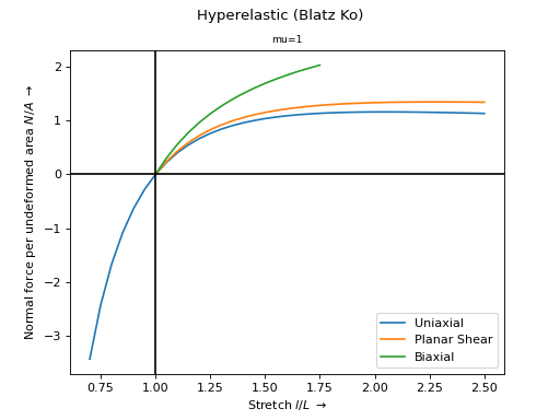
felupe.constitution.tensortrax.models.hyperelastic.blatz_ko(C, mu)[ソース]#

Strain energy function of the Blatz-Ko isotropic hyperelastic foam material formulation [1]_.

パラメータ:

C (tensortrax.Tensor or jax.Array) -- Right Cauchy-Green deformation tensor.
mu (float) -- The shear modulus.

メモ

The Poisson ratio of the Blatz-Ko model formulation is \(\nu = 0.25\). The strain energy function is given in Eq. (25)

(25)#\[\psi = \frac{\mu}{2} \left(\frac{I_2}{I_3} + 2 \sqrt{I_3} - 5 \right)\]

The shear modulus \(\mu\) is related to young's modulus as denoted in Eq. (26).

(26)#\[\mu = \frac{2 E}{5}\]

サンプル

First, choose the desired automatic differentiation backend

>>> # import felupe.constitution.jax as mat
>>> import felupe.constitution.tensortrax as mat

and create the hyperelastic material.

>>> umat = mat.Hyperelastic(mat.models.hyperelastic.blatz_ko, mu=1.0)
>>> ax = umat.plot()

参照

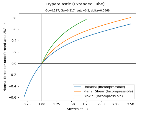
felupe.constitution.tensortrax.models.hyperelastic.extended_tube(C, Gc, delta, Ge, beta)[ソース]#

Strain energy function of the isotropic hyperelastic Extended Tube [1]_ material formulation.

パラメータ:

C (tensortrax.Tensor or jax.Array) -- Right Cauchy-Green deformation tensor.
Gc (float) -- Cross-link contribution to the initial shear modulus.
delta (float) -- Finite extension parameter of the polymer strands.
Ge (float) -- Constraint contribution to the initial shear modulus.
beta (float) -- Global rearrangements of cross-links upon deformation (release of topological constraints).

メモ

The strain energy function is given in Eq. (27)

(27)#\[\psi = \frac{G_c}{2} \left[ \frac{\left( 1 - \delta^2 \right) \left( \hat{I}_1 - 3 \right)}{1 - \delta^2 \left( \hat{I}_1 - 3 \right)} + \ln \left( 1 - \delta^2 \left( \hat{I}_1 - 3 \right) \right) \right] + \frac{2 G_e}{\beta^2} \left( \hat{\lambda}_1^{-\beta} + \hat{\lambda}_2^{-\beta} + \hat{\lambda}_3^{-\beta} - 3 \right)\]

with the first main invariant of the distortional part of the right Cauchy-Green deformation tensor as given in Eq. (28)

(28)#\[\hat{I}_1 = J^{-2/3} \text{tr}\left( \boldsymbol{C} \right)\]

and the principal stretches, obtained from the distortional part of the right Cauchy-Green deformation tensor, see Eq. (29).

(29)#\[ \begin{align}\begin{aligned}\lambda^2_\alpha &= \text{eigvals}\left( \boldsymbol{C} \right)\\\hat{\lambda}_\alpha &= J^{-1/3} \lambda_\alpha\end{aligned}\end{align} \]

The initial shear modulus results from the sum of the cross-link and the constraint contributions to the total initial shear modulus as denoted in Eq. (30).

(30)#\[\mu = G_e + G_c\]

サンプル

First, choose the desired automatic differentiation backend

>>> # import felupe.constitution.jax as mat
>>> import felupe.constitution.tensortrax as mat

and create the hyperelastic material.

>>> umat = mat.Hyperelastic(
...     mat.models.hyperelastic.extended_tube,
...     Gc=0.1867,
...     Ge=0.2169,
...     beta=0.2,
...     delta=0.09693,
... )
>>> ax = umat.plot(incompressible=True)

参照

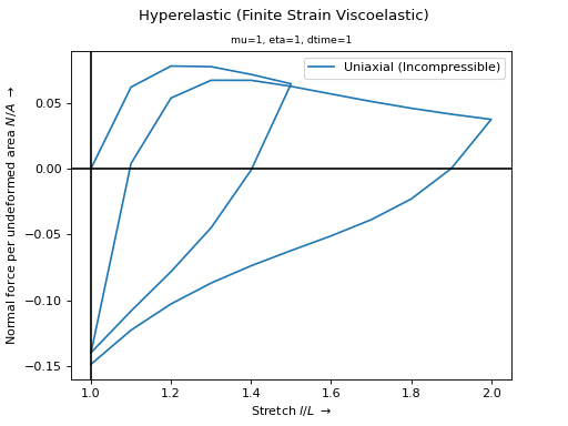
felupe.constitution.tensortrax.models.hyperelastic.finite_strain_viscoelastic(C, Cin, mu, eta, dtime)[ソース]#

Multiplicative finite strain viscoelastic [1]_ material formulation.

メモ

The material formulation is built upon the multiplicative decomposition of the distortional part of the deformation gradient tensor into an elastic and an inelastic part, see Eq. (31).

(31)#\[ \begin{align}\begin{aligned}\hat{\boldsymbol{F}} &= \boldsymbol{F}_e \boldsymbol{F}_i \ (= \hat{\boldsymbol{F}_e} \boldsymbol{F}_i)\\\boldsymbol{C}_e &= \boldsymbol{F}_e^T \boldsymbol{F}_e\\\boldsymbol{C}_i &= \boldsymbol{F}_i^T \boldsymbol{F}_i\\\text{tr}\left( \boldsymbol{C}_e \right) &= \text{tr}\left( \hat{\boldsymbol{C}} \boldsymbol{C}_i^{-1} \right)\end{aligned}\end{align} \]

The components of the inelastic right Cauchy-Green deformation tensor are used as state variables with the evolution equation and its explicit update formula as given in Eq. (32) [1]_. The elastic part of the multiplicative decomposition of the deformation gradient tensor is also enforced to be an unimodular tensor which leads to the constraint \(\det(\boldsymbol{F_i})=1\). Hence, the inelastic right Cauchy-Green deformation tensor must be an unimodular tensor \(\det(\boldsymbol{C_i})=1\).

(32)#\[ \begin{align}\begin{aligned}\dot{\boldsymbol{C}}_i &= \frac{\mu}{\eta}\ \hat{\boldsymbol{C}}\\\boldsymbol{C}_i &= \hat{\overline{\boldsymbol{C}_{i,n} + \frac{\Delta t \mu}{\eta} \hat{\boldsymbol{C}}}}\end{aligned}\end{align} \]

The distortional part of the strain energy density per unit undeformed volume is assumed to be of a Neo-Hookean form, see Eq. (33).

(33)#\[\hat{\psi} = \frac{\mu}{2} \left( \text{tr}\left( \hat{\boldsymbol{C}} \boldsymbol{C}_i^{-1} \right) - 3 \right)\]

サンプル

>>> import felupe as fem
>>>
>>> umat = fem.Hyperelastic(
...     fem.finite_strain_viscoelastic, mu=1.0, eta=1.0, dtime=1.0, nstatevars=6
... )
>>> ax = umat.plot(
...    incompressible=True,
...    ux=fem.math.linsteps([1, 1.5, 1, 2, 1], num=[5, 5, 10, 10]),
...    ps=None,
...    bx=None,
... )

参照

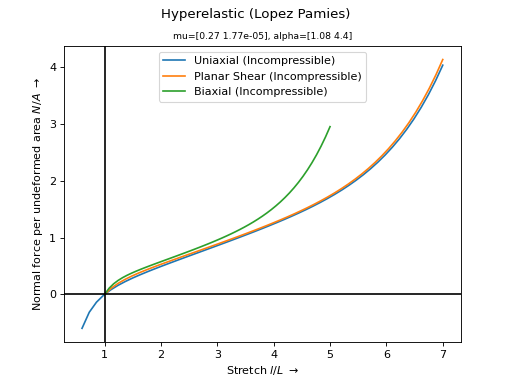
felupe.constitution.tensortrax.models.hyperelastic.lopez_pamies(C, mu, alpha)[ソース]#

Strain energy function of the isotropic hyperelastic Lopez-Pamies material formulation [1]_.

パラメータ:

C (tensortrax.Tensor) -- Right Cauchy-Green deformation tensor.
mu (list of float) -- List of moduli.
alpha (list of float) -- List of invariant exponents.

メモ

The strain energy function is given in Eq. (34)

(34)#\[\psi = \sum_{r=1}^M \frac{3^{1-\alpha_r}}{2 \alpha_r} \mu_r \left( \hat{I}_1^{\alpha_r} - 3^{\alpha_r} \right)\]

with the first main invariant of the distortional part of the right Cauchy-Green deformation tensor, see Eq. (35).

(35)#\[\hat{I}_1 = J^{-2/3} \text{tr}\left( \boldsymbol{C} \right)\]

The sum of the moduli \(\mu_r\) is equal to the initial shear modulus \(\mu\), see Eq. (36).

(36)#\[\mu = \sum_r \mu_r\]

サンプル

>>> import felupe as fem
>>>
>>> umat = fem.Hyperelastic(
...     fem.lopez_pamies, mu=[0.2699,  0.00001771], alpha=[1.08, 4.40]
... )
>>>
>>> ux = fem.math.linsteps([0.6, 7], num=50)
>>> ps = fem.math.linsteps([1, 7], num=50)
>>> bx = fem.math.linsteps([1, 5], num=50)
>>>
>>> ax = umat.plot(ux=ux, ps=ps, bx=bx, incompressible=True)

参照

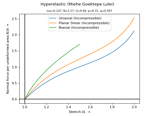
felupe.constitution.tensortrax.models.hyperelastic.miehe_goektepe_lulei(C, mu, N, U, p, q)[ソース]#

Strain energy function of the isotropic hyperelastic micro-sphere model formulation [1]_.

パラメータ:

C (tensortrax.Tensor or jax.Array) -- Right Cauchy-Green deformation tensor.
mu (float) -- Shear modulus (ground state stiffness).
N (float) -- Number of chain segments (chain locking response).
U (float) -- Tube geometry parameter (3D locking characteristics).
p (float) -- Non-affine stretch parameter (additional constraint stiffness).
q (float) -- Non-affine tube parameter (shape of constraint stress).

サンプル

First, choose the desired automatic differentiation backend

>>> # import felupe.constitution.jax as mat
>>> import felupe.constitution.tensortrax as mat

and create the hyperelastic material.

>>> import felupe as fem
>>>
>>> umat = mat.Hyperelastic(
...     mat.models.hyperelastic.miehe_goektepe_lulei,
...     mu=0.1475,
...     N=3.273,
...     p=9.31,
...     U=9.94,
...     q=0.567,
... )
>>> ux = ps = fem.math.linsteps([1, 2], num=50)
>>> bx = fem.math.linsteps([1, 1.5], num=50)
>>> ax = umat.plot(ux=ux, ps=ps, bx=bx, incompressible=True)

参照

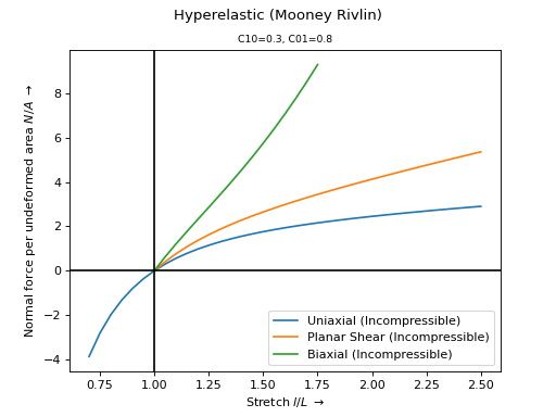
felupe.constitution.tensortrax.models.hyperelastic.mooney_rivlin(C, C10, C01)[ソース]#

Strain energy function of the isotropic hyperelastic Mooney-Rivlin material formulation.

パラメータ:

C (tensortrax.Tensor or jax.Array) -- Right Cauchy-Green deformation tensor.
C10 (float) -- First material parameter associated to the first invariant.
C01 (float) -- Second material parameter associated to the second invariant.

メモ

The strain energy function is given in Eq. (37)

(37)#\[\psi = C_{10} \left(\hat{I}_1 - 3 \right) + C_{01} \left(\hat{I}_2 - 3 \right)\]

with the first and second main invariant of the distortional part of the right Cauchy-Green deformation tensor, see Eq. (38).

(38)#\[ \begin{align}\begin{aligned}\hat{I}_1 &= J^{-2/3} \text{tr}\left( \boldsymbol{C} \right)\\\hat{I}_2 &= J^{-4/3} \frac{1}{2} \left( \text{tr}\left(\boldsymbol{C}\right)^2 - \text{tr}\left(\boldsymbol{C}^2\right) \right)\end{aligned}\end{align} \]

The doubled sum of both material parameters is equal to the shear modulus \(\mu\) as denoted in Eq. (39).

(39)#\[\mu = 2 \left( C_{10} + C_{01} \right)\]

サンプル

First, choose the desired automatic differentiation backend

>>> # import felupe.constitution.jax as mat
>>> import felupe.constitution.tensortrax as mat

and create the hyperelastic material.

>>> umat = mat.Hyperelastic(
...     mat.models.hyperelastic.mooney_rivlin, C10=0.3, C01=0.8
... )
>>> ax = umat.plot(incompressible=True)

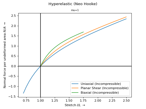
felupe.constitution.tensortrax.models.hyperelastic.neo_hooke(C, mu)[ソース]#

Strain energy function of the isotropic hyperelastic Neo-Hookean material formulation.

パラメータ:

C (tensortrax.Tensor or jax.Array) -- Right Cauchy-Green deformation tensor.
mu (float) -- Shear modulus.

メモ

The strain energy function is given in Eq. (40).

(40)#\[\psi = \frac{\mu}{2} \left(\text{tr}\left(\hat{\boldsymbol{C}}\right) - 3\right)\]

サンプル

First, choose the desired automatic differentiation backend

>>> # import felupe.constitution.jax as mat
>>> import felupe.constitution.tensortrax as mat

and create the hyperelastic material.

>>> umat = mat.Hyperelastic(mat.models.hyperelastic.neo_hooke, mu=1.0)
>>> ax = umat.plot(incompressible=True)

felupe.constitution.tensortrax.models.hyperelastic.ogden(C, mu, alpha)[ソース]#

Strain energy function of the isotropic hyperelastic Ogden material formulation.

パラメータ:

C (tensortrax.Tensor or jax.Array) -- Right Cauchy-Green deformation tensor.
mu (list of float) -- List of moduli.
alpha (list of float) -- List of stretch exponents.

メモ

The strain energy function is given in Eq. (41)

(41)#\[\psi = \sum_i \frac{2 \mu_i}{\alpha^2_i} \left( \lambda_1^{\alpha_i} + \lambda_2^{\alpha_i} + \lambda_3^{\alpha_i} - 3 \right)\]

The sum of the moduli \(\mu_i\) is equal to the initial shear modulus \(\mu\), see Eq. (42).

(42)#\[\mu = \sum_i \mu_i\]

サンプル

>>> # import felupe.constitution.jax as mat
>>> import felupe.constitution.tensortrax as mat

>>> umat = mat.Hyperelastic(
...     mat.models.hyperelastic.ogden, mu=[1, 0.2], alpha=[1.7, -1.5]
... )
>>> ax = umat.plot(incompressible=True)

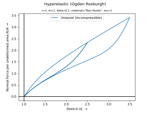
felupe.constitution.tensortrax.models.hyperelastic.ogden_roxburgh(C, Wmax_n, material, r, m, beta, **kwargs)[ソース]#

Ogden-Roxburgh Pseudo-Elastic material formulation for an isotropic treatment of the load-history dependent Mullins-softening of rubber-like materials.

パラメータ:

C (tensortrax.Tensor) -- Right Cauchy-Green deformation tensor.
Wmax_n (ndarray) -- State variable: value of the maximum strain energy density in load-history from the previous solution.
material (callable) -- Isotropic strain-energy density function. Optional keyword arguments are passed to material.
r (float) -- Reciprocal value of the maximum relative amount of softening. i.e. r=3 means the shear modulus of the base material scales down from \(1\) (no softening) to \(1 - 1/3 = 2/3\) (maximum softening).
m (float) -- The initial Mullins softening modulus.
beta (float) -- Maximum deformation-dependent part of the Mullins softening modulus.
**kwargs (dict) -- Optional keyword arguments are passed to the isotropic strain energy density function material.
warning:: (..) -- The keyword arguments of material must not include the names r, m and beta.

メモ

The pseudo-elastic strain energy density function \(\widetilde{\psi}\) and the Mullins-effect related evolution equation are given in Eq. (43). The variation of the functional \(\phi\) is defined in such a way that the term \(\delta \eta \ \hat{\psi}\) is canceled in the variation of the strain energy function \(\delta \psi\). The evolution equation \(\eta\) acts as a deformation and deformation-history dependent scaling factor on the variation of the distortional part of the strain energy density function.

(43)#\[ \begin{align}\begin{aligned}\widetilde{\psi} &= \eta \hat{\psi} + \phi\\\eta(\hat{\psi}, \hat{\psi}_\text{max}) &= 1 - \frac{1}{r} \text{erf} \left( \frac{\hat{\psi}_\text{max} - \psi}{m + \beta~\hat{\psi}_\text{max}} \right)\\\delta \phi &= -\delta \eta \ \hat{\psi}\\\delta \widetilde{\psi} &= \eta \ \delta \hat{\psi}\end{aligned}\end{align} \]

サンプル

>>> import felupe as fem
>>>
>>> umat = fem.Hyperelastic(
...     fem.ogden_roxburgh,
...     material=fem.neo_hooke,
...     r=3,
...     m=1,
...     beta=0.1,
...     mu=1,
...     nstatevars=1
... )
>>> ux = fem.math.linsteps(
...     [1, 2.5, 1, 3.5, 1], num=[15, 15, 25, 25]
... )
>>> ax = umat.plot(ux=ux, bx=None, ps=None, incompressible=True)

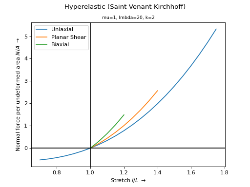
felupe.constitution.tensortrax.models.hyperelastic.saint_venant_kirchhoff(C, mu, lmbda, k=2)[ソース]#

Strain energy function of the isotropic hyperelastic Saint-Venant Kirchhoff material formulation.

パラメータ:

C (tensortrax.Tensor) -- Right Cauchy-Green deformation tensor.
mu (float) -- Second Lamé constant (shear modulus).
lmbda (float) -- First Lamé constant (shear modulus).
k (float, optional) -- Strain exponent (default is 2). If 2, the Green-Lagrange strain measure is used. For any other value, the family of Seth-Hill strains is used.

メモ

The strain energy function is given in Eq. (44)

(44)#\[\psi = \mu I_2 + \lambda \frac{I_1^2}{2}\]

with the first and second invariant of the Green-Lagrange strain tensor \(\boldsymbol{E} = \frac{1}{2} (\boldsymbol{C} - \boldsymbol{1})\), see Eq. (45).

(45)#\[ \begin{align}\begin{aligned}I_1 &= \text{tr}\left( \boldsymbol{E} \right)\\I_2 &= \boldsymbol{E} : \boldsymbol{E}\end{aligned}\end{align} \]

サンプル

警告

The Saint-Venant Kirchhoff material formulation is unstable for large strains.

>>> import felupe as fem
>>>
>>> umat = fem.Hyperelastic(fem.saint_venant_kirchhoff, mu=1.0, lmbda=20.0)
>>> ax = umat.plot(incompressible=False)

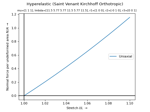
felupe.constitution.tensortrax.models.hyperelastic.saint_venant_kirchhoff_orthotropic(C, mu, lmbda, r1, r2, r3=None, k=2)[ソース]#

Strain energy function of the orthotropic hyperelastic Saint-Venant Kirchhoff material formulation.

パラメータ:

C (tensortrax.Tensor) -- Right Cauchy-Green deformation tensor.
mu (list of float) -- List of the three second Lamé parameters \(\mu_1,\mu_2, \mu_3\).
lmbda (list of float) -- List of six (upper triangle) first Lamé parameters \(\lambda_{11}, \lambda_{12}, \lambda_{13}, \lambda_{22}, \lambda_{23}, \lambda_{33}\).
r1 (list of float) -- First normal vector of planes of symmetry.
r2 (list of float) -- Second normal vector of planes of symmetry.
r3 (list of float or None, optional) -- Third normal vector of planes of symmetry. If None, the third normal vector is evaluated as \(r_1 \times r_2\). Default is None.
k (float, optional) -- Strain exponent (default is 2). If 2, the Green-Lagrange strain measure is used. For any other value, the family of Seth-Hill strains is used.

メモ

The strain energy function is given in Eq. (46)

(46)#\[\psi = \sum_{a=1}^3 \mu_a \boldsymbol{E} : \boldsymbol{r}_a \otimes \boldsymbol{r}_a + \sum_{a=1}^3 \sum_{b=1}^3 \frac{\lambda_{ab}}{2} \left(\boldsymbol{E} : \boldsymbol{r}_a \otimes \boldsymbol{r}_a \right) \left(\boldsymbol{E} : \boldsymbol{r}_b \otimes \boldsymbol{r}_b \right)\]

サンプル

警告

The orthotropic Saint-Venant Kirchhoff material formulation is unstable for large strains.

>>> import felupe.constitution.tensortrax as mat
>>> import felupe as fem
>>>
>>> r = fem.math.rotation_matrix(0, axis=2)
>>> lmbda, mu = fem.constitution.lame_converter_orthotropic(
...     E=[10, 10, 10],
...     nu=[0.3, 0.3, 0.3],
...     G=[1, 1, 1],
... )
>>> umat = mat.Hyperelastic(
...     mat.models.hyperelastic.saint_venant_kirchhoff_orthotropic,
...     mu=mu,
...     lmbda=lmbda,
...     r1=r[:, 0],
...     r2=r[:, 1],
...     r3=r[:, 2],
... )
>>> ax = umat.plot(ux=fem.math.linsteps([1, 1.1], num=10), ps=None, bx=None)

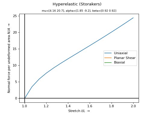
felupe.constitution.tensortrax.models.hyperelastic.storakers(C, mu, alpha, beta)[ソース]#

Strain energy function of the Storåkers isotropic hyperelastic foam material formulation [1]_.

パラメータ:

C (tensortrax.Tensor or jax.Array) -- Right Cauchy-Green deformation tensor.
mu (list of float) -- List of moduli.
alpha (list of float) -- List of stretch exponents.
beta (list of float) -- List of coefficients for the degree of compressibility.

メモ

The strain energy function is given in Eq. (47)

(47)#\[\psi = \sum_i \frac{2 \mu_i}{\alpha^2_i} \left[ \lambda_1^{\alpha_i} + \lambda_2^{\alpha_i} + \lambda_3^{\alpha_i} - 3 + \frac{1}{\beta_i} \left( J^{-\alpha_i \beta_i} - 1 \right) \right]\]

The sum of the moduli \(\mu_i\) is equal to the initial shear modulus \(\mu\), see Eq. (48),

(48)#\[\mu = \sum_i \mu_i\]

and the initial bulk modulus is given in Eq. (49).

(49)#\[K = \sum_i 2 \mu_i \left( \frac{1}{3} + \beta_i \right)\]

サンプル

First, choose the desired automatic differentiation backend

>>> # import felupe.constitution.jax as mat
>>> import felupe.constitution.tensortrax as mat

and create the hyperelastic material.

>>> import felupe as fem
>>>
>>> umat = mat.Hyperelastic(
...     mat.models.hyperelastic.storakers,
...     mu=[4.5 * (1.85 / 2), -4.5 * (-9.2 / 2)],
...     alpha=[1.85, -9.2],
...     beta=[0.92, 0.92],
... )
>>> ax = umat.plot(
...     ux=fem.math.linsteps([1, 2], 15),
...     ps=fem.math.linsteps([1, 1], 15),
...     bx=fem.math.linsteps([1, 1], 9),
... )

参照

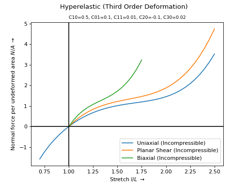
felupe.constitution.tensortrax.models.hyperelastic.third_order_deformation(C, C10, C01, C11, C20, C30)[ソース]#

Strain energy function of the isotropic hyperelastic Third-Order-Deformation material formulation.

パラメータ:

C (tensortrax.Tensor or jax.Array) -- Right Cauchy-Green deformation tensor.
C10 (float) -- Material parameter associated to the linear term of the first invariant.
C01 (float) -- Material parameter associated to the linear term of the second invariant.
C11 (float) -- Material parameter associated to the mixed term of the first and second invariant.
C20 (float) -- Material parameter associated to the quadratic term of the first invariant.
C30 (float) -- Material parameter associated to the cubic term of the first invariant.

メモ

The strain energy function is given in Eq. (50)

(50)#\[ \begin{align}\begin{aligned}\psi &= C_{10} \left(\hat{I}_1 - 3 \right) + C_{01} \left(\hat{I}_2 - 3 \right) + C_{11} \left(\hat{I}_1 - 3 \right) \left(\hat{I}_2 - 3 \right)\\ &+ C_{20} \left(\hat{I}_1 - 3 \right)^2 + C_{30} \left(\hat{I}_1 - 3 \right)^3\end{aligned}\end{align} \]

with the first and second main invariant of the distortional part of the right Cauchy-Green deformation tensor, see Eq. (51).

(51)#\[ \begin{align}\begin{aligned}\hat{I}_1 &= J^{-2/3} \text{tr}\left( \boldsymbol{C} \right)\\\hat{I}_2 &= J^{-4/3} \frac{1}{2} \left( \text{tr}\left(\boldsymbol{C}\right)^2 - \text{tr}\left(\boldsymbol{C}^2\right) \right)\end{aligned}\end{align} \]

The doubled sum of the material parameters \(C_{10}\) and \(C_{01}\) is equal to the initial shear modulus \(\mu\) as denoted in Eq. (52).

(52)#\[\mu = 2 \left( C_{10} + C_{01} \right)\]

サンプル

First, choose the desired automatic differentiation backend

>>> # import felupe.constitution.jax as mat
>>> import felupe.constitution.tensortrax as mat

and create the hyperelastic material.

>>> umat = mat.Hyperelastic(
...     mat.models.hyperelastic.third_order_deformation,
...     C10=0.5,
...     C01=0.1,
...     C11=0.01,
...     C20=-0.1,
...     C30=0.02,
... )
>>> ax = umat.plot(incompressible=True)

felupe.constitution.tensortrax.models.hyperelastic.van_der_waals(C, mu, limit, a, beta)[ソース]#

Strain energy function of the Van der Waals [1]_ material formulation.

パラメータ:

C (tensortrax.Tensor or jax.Array) -- Right Cauchy-Green deformation tensor.
mu (float) -- Initial shear modulus.
limit (float) -- Limiting stretch \(\lambda_m\) at which the polymer chain network becomes locked.
a (float) -- Attractive interactions between the quasi-particles.
beta (float) -- Mixed-Invariant factor: 0 for pure I1- and 1 for pure I2-contribution.

サンプル

First, choose the desired automatic differentiation backend

>>> # import felupe.constitution.jax as mat
>>> import felupe.constitution.tensortrax as mat

and create the hyperelastic material.

>>> umat = mat.Hyperelastic(
...     mat.models.hyperelastic.van_der_waals,
...     mu=1.0,
...     beta=0.1,
...     a=0.5,
...     limit=5.0
... )
>>> ax = umat.plot(incompressible=True)

参照

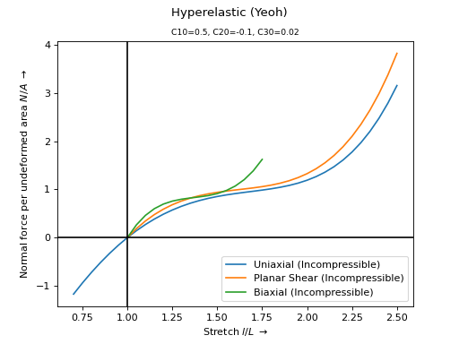
felupe.constitution.tensortrax.models.hyperelastic.yeoh(C, C10, C20, C30)[ソース]#

Strain energy function of the isotropic hyperelastic Yeoh material formulation.

パラメータ:

C (tensortrax.Tensor or jax.Array) -- Right Cauchy-Green deformation tensor.
C10 (float) -- Material parameter associated to the linear term of the first invariant.
C20 (float) -- Material parameter associated to the quadratic term of the first invariant.
C30 (float) -- Material parameter associated to the cubic term of the first invariant.

メモ

The strain energy function is given in Eq. (53)

(53)#\[\psi = C_{10} \left(\hat{I}_1 - 3 \right) + C_{20} \left(\hat{I}_1 - 3 \right)^2 + C_{30} \left(\hat{I}_1 - 3 \right)^3\]

with the first main invariant of the distortional part of the right Cauchy-Green deformation tensor, see Eq. (54).

(54)#\[\hat{I}_1 = J^{-2/3} \text{tr}\left( \boldsymbol{C} \right)\]

The \(C_{10}\) material parameter is equal to half the initial shear modulus \(\mu\) as denoted in Eq. (55).

(55)#\[\mu = 2 C_{10}\]

サンプル

First, choose the desired automatic differentiation backend

>>> # import felupe.constitution.jax as mat
>>> import felupe.constitution.tensortrax as mat

and create the hyperelastic material.

>>> umat = mat.Hyperelastic(
...     mat.models.hyperelastic.yeoh, C10=0.5, C20=-0.1, C30=0.02
... )
>>> ax = umat.plot(incompressible=True)

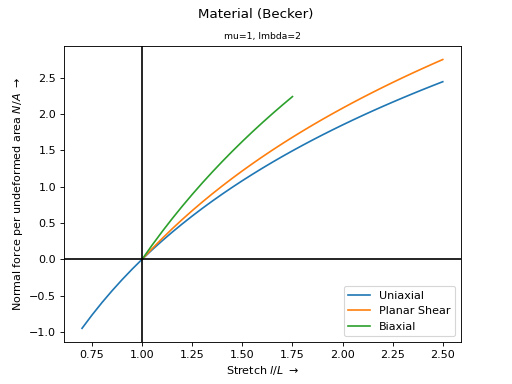
felupe.constitution.tensortrax.models.lagrange.becker(F, mu, lmbda)[ソース]#

Second Piola-Kirchhoff stress tensor of Becker's logarithmic material model formulation [1]_ [2]_.

パラメータ:

F (tensortrax.Tensor or jax.Array) -- Deformation gradient tensor.
mu (float) -- Shear modulus (second Lamé parameter).
lmbda (float) -- First Lamé parameter.

戻り値:

S -- Second Piola-Kirchhoff stress tensor.

戻り値の型:

tensortrax.Tensor or jax.Array

メモ

This logarithmic material model formulation utilizes a linear-elastic stress-strain formulation for the Biot stress tensor, based on the Lagrangian logarithmic strain tensor, see Eq. (56).

(56)#\[\boldsymbol{T} = 2 \mu \ \ln \boldsymbol{U} + \lambda \ \operatorname{tr}(\ln \boldsymbol{U}) \boldsymbol{1}\]

The second Piola-Kirchhoff stress tensor is then obtained from the Biot stress tensor, see Eq. (57).

(57)#\[\boldsymbol{S} = \boldsymbol{U}^{-1} \boldsymbol{T}\]

サンプル

First, choose the desired automatic differentiation backend

>>> import felupe as fem
>>>
>>> # import felupe.constitution.jax as mat
>>> import felupe.constitution.tensortrax as mat

and create the material.

>>> umat = mat.Material(mat.models.lagrange.becker, mu=1.0, lmbda=2.0)
>>> ax = umat.plot()

参照

felupe.constitution.tensortrax.models.lagrange.morph(F, statevars, p)[ソース]#

Second Piola-Kirchhoff stress tensor of the MORPH model formulation [1]_.

パラメータ:

F (tensortrax.Tensor or jax.Array) -- Deformation gradient tensor.
statevars (array) -- Vector of stacked state variables (CTS, C, SA).
p (list of float) -- A list which contains the 8 material parameters.

メモ

The MORPH material model is implemented as a second Piola-Kirchhoff stress-based formulation with automatic differentiation. The Tresca invariant of the distortional part of the right Cauchy-Green deformation tensor is used as internal state variable, see Eq. (58).

警告

While the MORPH-material formulation captures the Mullins effect and quasi-static hysteresis effects of rubber mixtures very nicely, it has been observed to be unstable for medium- to highly-distorted states of deformation.

(58)#\[ \begin{align}\begin{aligned}\boldsymbol{C} &= \boldsymbol{F}^T \boldsymbol{F}\\I_3 &= \det (\boldsymbol{C})\\\hat{\boldsymbol{C}} &= I_3^{-1/3} \boldsymbol{C}\\\hat{\lambda}^2_\alpha &= \text{eigvals}(\hat{\boldsymbol{C}})\\\hat{C}_T &= \max \left( \hat{\lambda}^2_\alpha - \hat{\lambda}^2_\beta \right)\\\hat{C}_T^S &= \max \left( \hat{C}_T, \hat{C}_{T,n}^S \right)\end{aligned}\end{align} \]

A sigmoid-function is used inside the deformation-dependent variables \(\alpha\), \(\beta\) and \(\gamma\), see Eq. (59).

(59)#\[ \begin{align}\begin{aligned}f(x) &= \frac{1}{\sqrt{1 + x^2}}\\\alpha &= p_1 + p_2 \ f(p_3\ C_T^S)\\\beta &= p_4\ f(p_3\ C_T^S)\\\gamma &= p_5\ C_T^S\ \left( 1 - f\left(\frac{C_T^S}{p_6}\right) \right)\end{aligned}\end{align} \]

The rate of deformation is described by the Lagrangian tensor and its Tresca- invariant, see Eq. (60).

注釈

It is important to evaluate the incremental right Cauchy-Green tensor by the difference of the final and the previous state of deformation, not by its variation with respect to the deformation gradient tensor.

(60)#\[ \begin{align}\begin{aligned}\hat{\boldsymbol{L}} &= \text{sym}\left( \text{dev}(\boldsymbol{C}^{-1} \Delta\boldsymbol{C}) \right) \hat{\boldsymbol{C}}\\\lambda_{\hat{\boldsymbol{L}}, \alpha} &= \text{eigvals}(\hat{\boldsymbol{L}})\\\hat{L}_T &= \max \left( \lambda_{\hat{\boldsymbol{L}}, \alpha}-\lambda_{\hat{\boldsymbol{L}}, \beta} \right)\\\Delta\boldsymbol{C} &= \boldsymbol{C} - \boldsymbol{C}_n\end{aligned}\end{align} \]

The additional stresses evolve between the limiting stresses, see Eq. (61). The additional deviatoric-enforcement terms [1]_ are neglected in this implementation.

(61)#\[ \begin{align}\begin{aligned}\boldsymbol{S}_L &= \left( \gamma \exp \left(p_7 \frac{\hat{\boldsymbol{L}}}{\hat{L}_T} \frac{\hat{C}_T}{\hat{C}_T^S} \right) + p8 \frac{\hat{\boldsymbol{L}}}{\hat{L}_T} \right) \boldsymbol{C}^{-1}\\\boldsymbol{S}_A &= \frac{ \boldsymbol{S}_{A,n} + \beta\ \hat{L}_T\ \boldsymbol{S}_L }{1 + \beta\ \hat{L}_T}\\\boldsymbol{S} &= 2 \alpha\ \text{dev}( \hat{\boldsymbol{C}} ) \boldsymbol{C}^{-1}+\text{dev}\left(\boldsymbol{S}_A\ \boldsymbol{C}\right) \boldsymbol{C}^{-1}\end{aligned}\end{align} \]

注釈

Only the upper-triangle entries of the symmetric stress-tensor state variables are stored in the solid body. Hence, it is necessary to extract such variables with tm.special.from_triu_1d() and export them as tm.special.triu_1d().

サンプル

First, choose the desired automatic differentiation backend

>>> import felupe as fem
>>>
>>> # import felupe.constitution.jax as mat
>>> import felupe.constitution.tensortrax as mat

and create the material.

>>> umat = mat.Material(
...     mat.models.lagrange.morph,
...     p=[0.039, 0.371, 0.174, 2.41, 0.0094, 6.84, 5.65, 0.244],
...     nstatevars=13,
... )
>>> ax = umat.plot(
...    incompressible=True,
...    ux=fem.math.linsteps(
...        # [1, 2, 1, 2.75, 1, 3.5, 1, 4.2, 1, 4.8, 1, 4.8, 1],
...        [1, 2.75, 1, 2.75],
...        num=20,
...    ),
...    ps=None,
...    bx=None,
... )

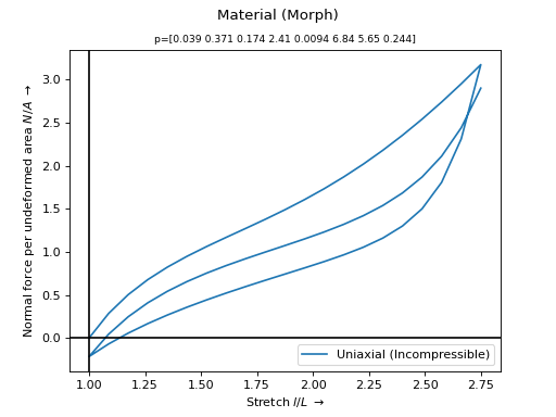
参照

参考

felupe.constitution.tensortrax.models.lagrange.morph_representative_directions: Strain energy function of the MORPH model formulation, implemented by the concept of representative directions.
felupe.constitution.jax.models.lagrange.morph_representative_directions: Strain energy function of the MORPH model formulation, implemented by the concept of representative directions.

felupe.constitution.tensortrax.models.lagrange.morph_representative_directions(F, statevars, p, ε=1e-06)[ソース]#

First Piola-Kirchhoff stress tensor of the MORPH model formulation [1]_, implemented by the concept of representative directions [2]_, [3].

パラメータ:

F (tensortrax.Tensor or jax.Array) -- Deformation gradient tensor.
statevars (array) -- Vector of stacked state variables (CTS, λ - 1, SA1, SA2).
p (list of float) -- A list which contains the 8 material parameters.
ε (float, optional) -- A small stabilization parameter (default is 1e-6).

サンプル

First, choose the desired automatic differentiation backend

>>> import felupe as fem
>>>
>>> # import felupe.constitution.jax as mat
>>> import felupe.constitution.tensortrax as mat

and create the material.

>>> umat = mat.Material(
...     mat.models.lagrange.morph_representative_directions,
...     p=[0.011, 0.408, 0.421, 6.85, 0.0056, 5.54, 5.84, 0.117],
...     nstatevars=84,
... )
>>> ax = umat.plot(
...    incompressible=True,
...    ux=fem.math.linsteps(
...        # [1, 2, 1, 2.75, 1, 3.5, 1, 4.2, 1, 4.8, 1, 4.8, 1],
...        [1, 2.75, 1, 2.75],
...        num=20,
...    ),
...    ps=None,
...    bx=None,
... )

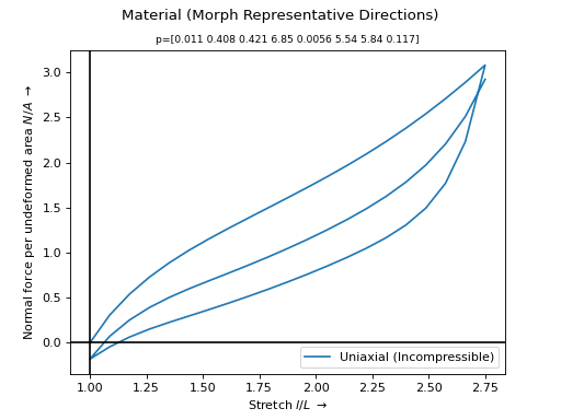
参照

参考

felupe.constitution.tensortrax.models.lagrange.morph: Strain energy function of the MORPH model formulation.
felupe.constitution.jax.models.lagrange.morph: Strain energy function of the MORPH model formulation.