Rotating Rubber Wheel

This example contains a simulation of a rotating rubber wheel in plane strain with the MORPH material model formulation [1]. While the rotation is increased, a constant vertical compression is applied to the rubber wheel by a contact on the bottom. The vertical reaction force is then carried out for the rotation angles. The MORPH material model is implemented as a second Piola- Kirchhoff stress-based formulation with automatic differentiation (JAX). The Tresca invariant of the distortional part of the right Cauchy-Green deformation tensor is used as internal state variable, see Eq. (1).

警告

While the MORPH-material formulation captures the Mullins effect and quasi-static hysteresis effects of rubber mixtures very nicely, it has been observed to be unstable for medium- to highly-distorted states of deformation. An alternative implementation by the method of representative directions provides better stability but is computationally more costly [2], [3].

(1)\[ \begin{align}\begin{aligned}\boldsymbol{C} &= \boldsymbol{F}^T \boldsymbol{F}\\I_3 &= \det (\boldsymbol{C})\\\hat{\boldsymbol{C}} &= I_3^{-1/3} \boldsymbol{C}\\\hat{\lambda}^2_\alpha &= \text{eigvals}(\hat{\boldsymbol{C}})\\\hat{C}_T &= \max \left( \hat{\lambda}^2_\alpha - \hat{\lambda}^2_\beta \right)\\\hat{C}_T^S &= \max \left( \hat{C}_T, \hat{C}_{T,n}^S \right)\end{aligned}\end{align} \]

A sigmoid-function is used inside the deformation-dependent variables \(\alpha\), \(\beta\) and \(\gamma\), see Eq. (2).

(2)\[ \begin{align}\begin{aligned}f(x) &= \frac{1}{\sqrt{1 + x^2}}\\\alpha &= p_1 + p_2 \ f(p_3\ C_T^S)\\\beta &= p_4\ f(p_3\ C_T^S)\\\gamma &= p_5\ C_T^S\ \left( 1 - f\left(\frac{C_T^S}{p_6}\right) \right)\end{aligned}\end{align} \]

The rate of deformation is described by the Lagrangian tensor and its Tresca-invariant, see Eq. (3).

注釈

It is important to evaluate the incremental right Cauchy-Green tensor by the difference of the final and the previous state of deformation, not by its variation with respect to the deformation gradient tensor.

(3)\[ \begin{align}\begin{aligned}\hat{\boldsymbol{L}} &= \text{sym}\left( \text{dev}(\boldsymbol{C}^{-1} \Delta\boldsymbol{C}) \right) \hat{\boldsymbol{C}}\\\lambda_{\hat{\boldsymbol{L}}, \alpha} &= \text{eigvals}(\hat{\boldsymbol{L}})\\\hat{L}_T &= \max \left( \lambda_{\hat{\boldsymbol{L}}, \alpha} - \lambda_{\hat{\boldsymbol{L}}, \beta} \right)\\\Delta\boldsymbol{C} &= \boldsymbol{C} - \boldsymbol{C}_n\end{aligned}\end{align} \]

The additional stresses evolve between the limiting stresses, see Eq. (4). The additional deviatoric-enforcement terms [1] are neglected in this example.

(4)\[ \begin{align}\begin{aligned}\boldsymbol{S}_L &= \left( \gamma \exp \left(p_7 \frac{\hat{\boldsymbol{L}}}{\hat{L}_T} \frac{\hat{C}_T}{\hat{C}_T^S} \right) + p8 \frac{\hat{\boldsymbol{L}}}{\hat{L}_T} \right) \boldsymbol{C}^{-1}\\\boldsymbol{S}_A &= \frac{ \boldsymbol{S}_{A,n} + \beta\ \hat{L}_T\ \boldsymbol{S}_L }{1 + \beta\ \hat{L}_T}\\\boldsymbol{S} &= 2 \alpha\ \text{dev}( \hat{\boldsymbol{C}} ) \boldsymbol{C}^{-1} + \text{dev}\left( \boldsymbol{S}_A\ \boldsymbol{C} \right) \boldsymbol{C}^{-1}\end{aligned}\end{align} \]

注釈

Only the upper-triangle entries of the symmetric stress-tensor state variables are stored in the solid body.

import jax.numpy as jnp
import numpy as np
from jax.scipy.linalg import expm

import felupe as fem
import felupe.constitution.jax as mat


def morph(F, statevars, p):
    "MORPH material model formulation."

    # right Cauchy-Green deformation tensor
    C = F.T @ F

    # extract old state variables
    CTSn = statevars[0]
    from_triu = lambda C: C[jnp.array([[0, 1, 2], [1, 3, 4], [2, 4, 5]])]
    Cn = from_triu(statevars[1:7])
    SAn = from_triu(statevars[7:13])

    # distortional part of right Cauchy-Green deformation tensor
    I3 = jnp.linalg.det(C)
    CG = C * I3 ** (-1 / 3)

    # inverse of and incremental right Cauchy-Green deformation tensor
    invC = jnp.linalg.inv(C)
    dC = C - Cn

    # eigenvalues of right Cauchy-Green deformation tensor (sorted in ascending order)
    ε = jnp.diag(jnp.array([1e-4, -1e-4, 0]))
    eigvalsh_ε = lambda C: jnp.linalg.eigvalsh(C + ε)
    λCG = eigvalsh_ε(CG)

    # Tresca invariant of distortional part of right Cauchy-Green deformation tensor
    CTG = λCG[-1] - λCG[0]

    # maximum Tresca invariant in load history
    CTS = jnp.maximum(CTG, CTSn)

    def sigmoid(x):
        "Algebraic sigmoid function."
        return 1 / jnp.sqrt(1 + x**2)

    # material parameters
    α = p[0] + p[1] * sigmoid(p[2] * CTS)
    β = p[3] * sigmoid(p[2] * CTS)
    γ = p[4] * CTS * (1 - sigmoid(CTS / p[5]))

    dev = lambda C: C - jnp.trace(C) / 3 * jnp.eye(3)
    sym = lambda C: (C + C.T) / 2

    LG = sym(dev(invC @ dC)) @ CG
    λLG = eigvalsh_ε(LG)
    LTG = λLG[-1] - λLG[0]

    # limiting stresses "L" and additional stresses "A"
    SL = (γ * expm(p[6] * LG / LTG * CTG / CTS) + p[7] * LG / LTG) @ invC
    SA = (SAn + β * LTG * SL) / (1 + β * LTG)

    # second Piola-Kirchhoff stress tensor
    S = 2 * α * dev(CG) @ invC + dev(SA @ C) @ invC

    # update the state variables
    i, j = jnp.triu_indices(3)
    to_triu = lambda C: C[i, j]
    statevars_new = jnp.concatenate([jnp.array([CTS]), to_triu(C), to_triu(SA)])

    return F @ S, statevars_new


umat = mat.Material(
    morph,
    p=[0.039, 0.371, 0.174, 2.41, 0.0094, 6.84, 5.65, 0.244],
    nstatevars=13,
)

注釈

The MORPH material model formulation is also available in FElupe, see morph (tensortrax) and morph (JAX).

The force-stress curves are shown for uniaxial incompressible tension cycles.

ux = fem.math.linsteps([1, 1.5, 1, 2, 1, 2.5, 1, 2.5], num=(5, 5, 10, 10, 15, 15, 15))
ax = umat.plot(
    ux=ux,
    bx=None,
    ps=None,
    incompressible=True,
)

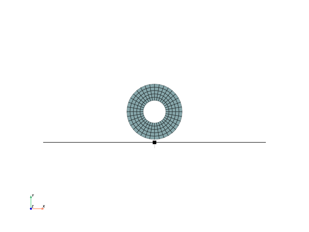
A mesh is created for the wheel with \(r=40\) mm and \(R=100\) mm.

mesh = fem.mesh.Line(a=40, b=100, n=6).revolve(37, phi=360)
mesh.add_points([0, -110])

x, y = mesh.points.T

A quad-region and a plane-strain displacement field are created. Mesh-points at \(r\) are added to the move-boundary condition. The displacements due to the rotation of the wheel are evaluated for each rotation angle. The center-point of the bottom-edge is moved vertically upwards by 20 mm to enforce a vertical reaction force in the rubber wheel.

region = fem.RegionQuad(mesh)
field = fem.FieldContainer([fem.FieldPlaneStrain(region, dim=2)])

mask = np.isclose(np.sqrt(x**2 + y**2), 40)
boundaries = {
    "move": fem.dof.Boundary(field[0], mask=mask),
    "bottom-x": fem.dof.Boundary(field[0], fy=-110, value=0, skip=(0, 1)),
    "bottom-y": fem.dof.Boundary(field[0], fy=-110, value=20, skip=(1, 0)),
}

angles_deg = fem.math.linsteps([0, 120], num=12)
move = []
for phi in angles_deg:
    center = mesh.points[boundaries["move"].points]
    center_rotated = fem.math.rotate_points(
        points=center,
        angle_deg=phi,
        axis=0,
        center=[0, 0],
    )
    move.append(center_rotated - center)

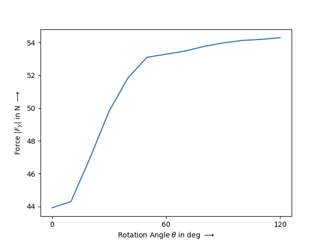
A nearly-incompressible solid body is created for the rubber. At the bottom, a contact plane is created. Both items are added to a step, which is further evaluated in a job. The vertical displacement of the bottom contact plane is applied in a preliminary job. Afterwards, the horizontal movement of the bottom contact plane is released and the second job is evaluated for the rotation of the wheel. The reaction forces are plotted for the successive rotation angles of the wheel.

solid = fem.SolidBodyNearlyIncompressible(umat, field, bulk=5000)
bottom = fem.ContactRigidPlane(
    field,
    points=np.arange(mesh.npoints)[np.isclose(np.sqrt(x**2 + y**2), 100)],
    centerpoint=-1,
    normal=(0, 1),
    friction=0.3,
    multiplier=40.0,
    multiplier_tangential=1.0,
)
plotter = bottom.plot(color="black", line_width=2, opacity=1.0, size=800)
mesh.plot(plotter=plotter).show()

step_compression = fem.Step(items=[solid, bottom], boundaries=boundaries)
job_compression = fem.Job(steps=[step_compression]).evaluate(tol=1e-1)

boundaries.pop("bottom-x")
step = fem.Step(
    items=[solid, bottom],
    ramp={boundaries["move"]: move},
    boundaries=boundaries,
)
job = fem.CharacteristicCurve(steps=[step], boundary=boundaries["move"])
job.evaluate(tol=1e-2)

fig, ax = job.plot(
    x=angles_deg.reshape(-1, 1),
    yaxis=1,
    yscale=-1,
    xlabel=r"Rotation Angle $\theta$ in deg $\longrightarrow$",
    ylabel=r"Force $|F_y|$ in N $\longrightarrow$",
)
ax.set_xticks(angles_deg[::6])

Static Scene

Interactive Scene

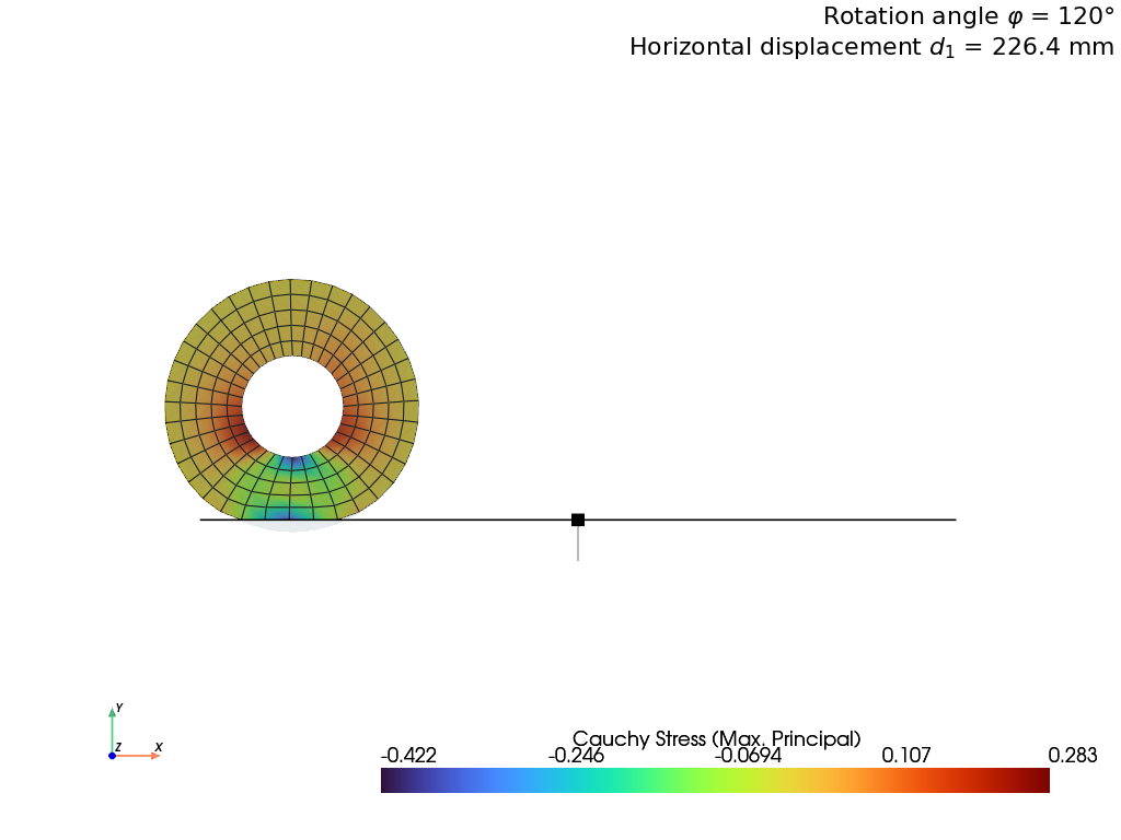
The resulting max. principal values of the Cauchy stresses are shown for the final rotation angle. As a result of friction, the bottom contact plane moves horizontally to the right.

plotter = bottom.plot(color="black", line_width=2, opacity=1.0, size=600)
plotter = solid.plot(
    "Principal Values of Cauchy Stress",
    plotter=plotter,
    project=fem.topoints,
)
plotter.add_text(
    rf"Rotation angle $\varphi$ = {angles_deg[-1]:.0f}°"
    "\n \n"
    rf"Horizontal displacement $d_1$ = {field[0].values[bottom.centerpoint][0]:.1f} mm",
    position="upper_right",
    font_size=12,
)
plotter.show()

Static Scene

Interactive Scene

参考資料

[1] (1,2)

D. Besdo and J. Ihlemann, "A phenomenological constitutive model for rubberlike materials and its numerical applications", International Journal of Plasticity, vol. 19, no. 7. Elsevier BV, pp. 1019–1036, Jul. 2003. doi: 10.1016/s0749-6419(02)00091-8.

[2]

M. Freund, "Verallgemeinerung eindimensionaler Materialmodelle für die Finite-Elemente-Methode", Dissertation, Technische Universität Chemnitz, Chemnitz, 2013.

[3]

C. Miehe, S. Göktepe and F. Lulei, "A micro-macro approach to rubber-like materials - Part I: the non-affine micro-sphere model of rubber elasticity", Journal of the Mechanics and Physics of Solids, vol. 52, no. 11. Elsevier BV, pp. 2617–2660, Nov. 2004. doi: 10.1016/j.jmps.2004.03.011.