Mixed-field hyperelasticity with quadratic triangles

A 90° section of a plane-strain circle is subjected to uniaxial compression by a vertically moved rigid top plate. A mixed-field formulation is used with quadratic triangles.

from functools import partial

import numpy as np

import felupe as fem

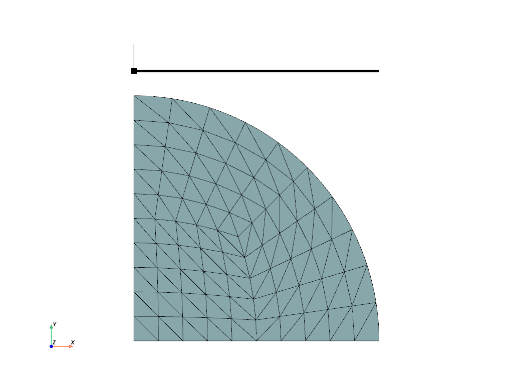
A 90° section of a circle with quadratic triangles is created. The midpoints are shifted to the outer radius. An additional point, used as center- (control-) point, is added to the mesh.

mesh = fem.Circle(n=6, sections=[0]).triangulate().add_midpoints_edges()
mask = np.isclose(mesh.x**2 + mesh.y**2, 1, atol=0.05)
mesh.points[mask] /= np.linalg.norm(mesh.points[mask], axis=1).reshape(-1, 1)
mesh.add_points([0, 1.1])

Let's create a region for quadratic triangles and a mixed-field container with two dual fields, one for the pressure and another one for the volume ratio. The dual fields are disconnected.

region = fem.RegionQuadraticTriangle(mesh)
field = fem.FieldsMixed(
    region, n=3, values=(0.0, 0.0, 1.0), planestrain=True, disconnect=True
)

# create a nearly-incompressible hyperelastic solid body and the rigid top plate
umat = fem.NearlyIncompressible(material=fem.NeoHooke(mu=1), bulk=5000)
solid = fem.SolidBody(umat=umat, field=field)
top = fem.ContactRigidPlane(
    field=field,
    points=np.arange(mesh.npoints)[np.isclose(mesh.x**2 + mesh.y**2, 1)],
    centerpoint=-1,
    normal=(0, -1),
    items=[solid],
    friction=0.5,
    multiplier=10,  # increase contact normal multiplier
    multiplier_tangential=2,  # increase contact tangential multiplier
)
kwargs = dict(line_width=5, opacity=1, sym=(True, False), size=2)
mesh.plot(nonlinear_subdivision=4, plotter=top.plot(**kwargs)).show()

Static Scene

Interactive Scene

A step is used containts the solid body and the rigid top plate as items. The rigid vertical movement of the top plate is applied in a ramped manner.

boundaries = fem.dof.symmetry(field[0])
boundaries["move"] = fem.Boundary(field[0], fy=1.1, skip=(1, 0))
move = fem.math.linsteps([0, -0.4], num=6)
ramp = {boundaries["move"]: move}
step = fem.Step(items=[solid, top], ramp=ramp, boundaries=boundaries)
job = fem.Job(steps=[step]).evaluate()

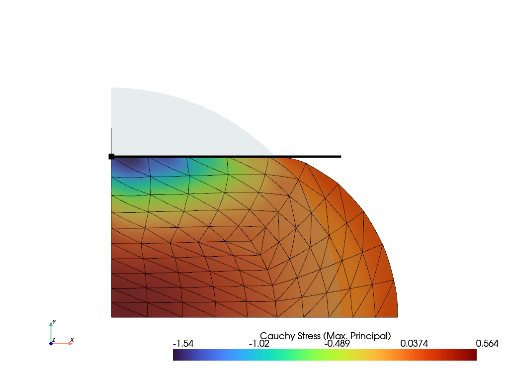
The maximum principal values of the Cauchy stress tensor are plotted. The cell-based means are projected to the mesh-points.

solid.plot(
    "Principal Values of Cauchy Stress",
    nonlinear_subdivision=4,
    plotter=top.plot(**kwargs),
    project=partial(fem.project, mean=True),
).show()

Static Scene

Interactive Scene