穴の開いたプレート#

A plate with length \(2L\), height \(2h\) and a hole with radius \(r\) is subjected to a uniaxial tension \(p=-100\) MPa. What is being looked for is the von Mises stress distribution and the concentration of normal stress \(\sigma_{11}\) over the hole.

../_images/ex02_plate-with-hole_sketch.svg

h = 1
L = 2
r = 0.3

import numpy as np

四角セルで穴のあいたメッシュ・プレートを作ってみましょう。プレートの1/4モデルのみを考えます。メッシュの生成は穴のエッジとトップラインの間の領域を埋めることで行われます。そして、この部分を複製し、ミラーリングして、別の長方形と統合します。

import felupe as fem

phi = np.linspace(1, 0.5, 21) * np.pi / 2

line = fem.mesh.Line(n=21)
curve = line.copy(points=r * np.vstack([np.cos(phi), np.sin(phi)]).T)
top = line.copy(points=np.vstack([np.linspace(0, h, 21), np.linspace(h, h, 21)]).T)

face = curve.fill_between(top, n=np.linspace(0, 1, 21) ** 1.3 * 2 - 1)
rect = fem.mesh.Rectangle(a=(h, 0), b=(L, h), n=21)
mesh = fem.mesh.concatenate([face, face.mirror(normal=[-1, 1, 0]), rect])
mesh = mesh.sweep(decimals=5)

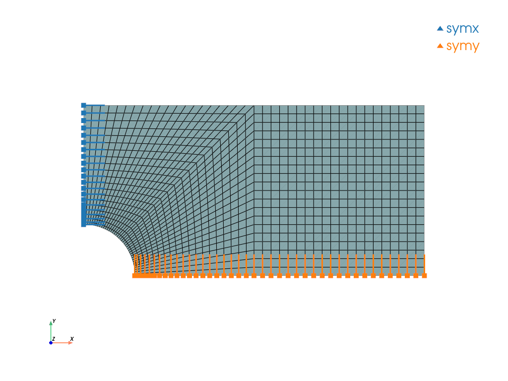
ベクトル値の変位場と組み合わせてメッシュ上に作成された数値4値領域がプレートを表します。対称面の境界条件は、変位場上に生成されます。

region = fem.RegionQuad(mesh)
displacement = fem.Field(region, dim=2)
field = fem.FieldContainer([displacement])

boundaries = fem.dof.symmetry(displacement)
boundaries.plot().show()

Static Scene

Interactive Scene

材料挙動は、平面応力問題のための組み込みの等方性線形弾性材料定式化によって定義されます。固体は、変位フィールドに線形弾性材料定式化を適用します。

umat = fem.LinearElasticPlaneStress(E=210000, nu=0.3)
solid = fem.SolidBody(umat, field)

The external uniaxial tension is applied by a pressure load on the right end at \(x=L\). Therefore, a boundary region in combination with a field has to be created at \(x=L\).

region_boundary = fem.RegionQuadBoundary(mesh, mask=mesh.points[:, 0] == L)
field_boundary = fem.FieldContainer([fem.Field(region_boundary, dim=2)])

load = fem.SolidBodyPressure(field_boundary, pressure=-100)

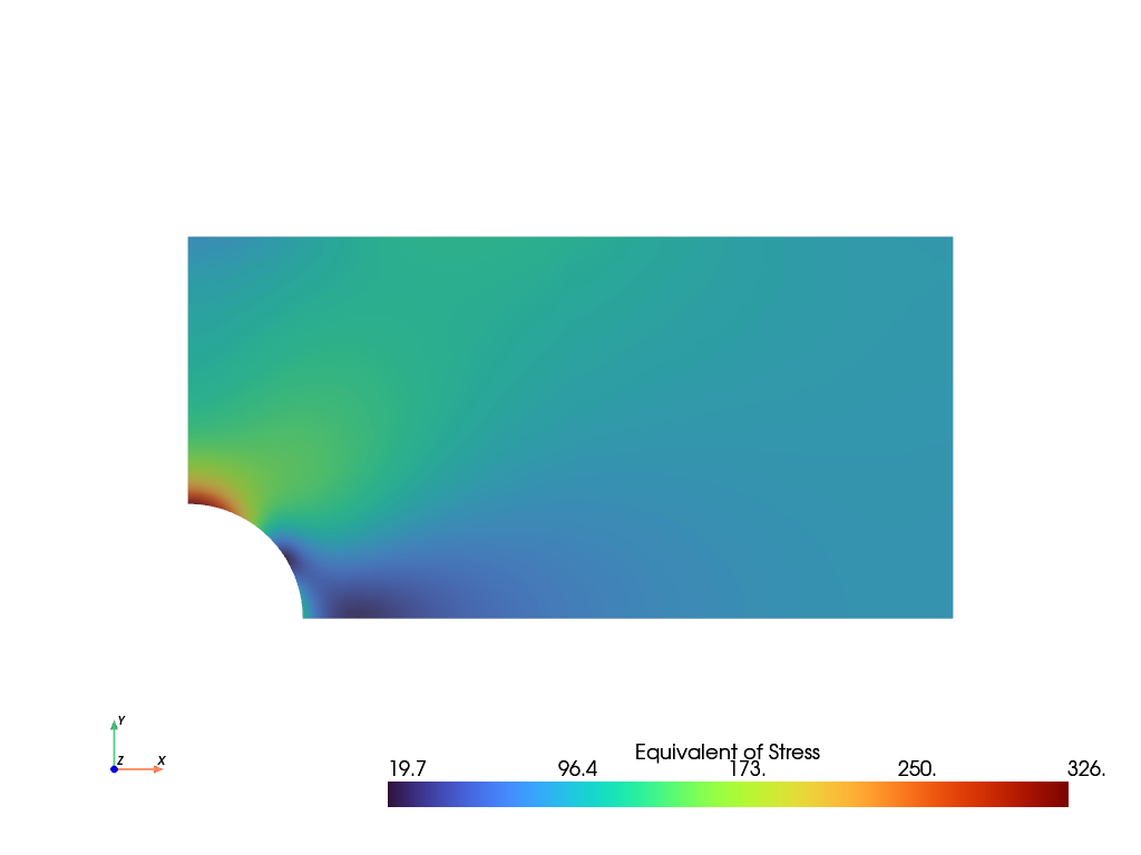
The simulation model is now ready to be solved. The equivalent von Mises stress will be plotted. For the two-dimensional case it is calculated by Eq. (1). Stresses, located at quadrature-points of cells, are shifted to and averaged at mesh- points.

(1)#\[\sigma_{vM} = \sqrt{\sigma_{11}^2 + \sigma_{22}^2 - \sigma_{11} \ \sigma_{22} + 3 \ \sigma_{12}^2}\]

step = fem.Step(items=[solid, load], boundaries=boundaries)
job = fem.Job(steps=[step]).evaluate()

solid.plot("Equivalent of Stress", show_edges=False, project=fem.topoints).show()

Static Scene

Interactive Scene

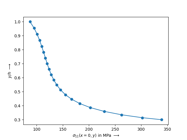
\(x=0\) の穴の法線応力分布 \(\sigma_{11}\) をmatplotlibでプロットします。

import matplotlib.pyplot as plt

plt.plot(
    fem.tools.project(solid.evaluate.stress(), region)[:, 0, 0][mesh.x == 0],
    mesh.points[:, 1][mesh.x == 0] / h,
    "o-",
)

plt.xlabel(r"$\sigma_{11}(x=0, y)$ in MPa $\longrightarrow$")
plt.ylabel(r"$y/h$ $\longrightarrow$")

Total running time of the script: (0 minutes 0.815 seconds)

Sphinx-Galleryによって生成されたギャラリー